Getting started with audio keyword spotting on the Raspberry Pi

by Chris Lovett

This tutorial guides you through the process of getting started with audio keyword spotting on your Raspberry Pi device. Unlike previous tutorials in this series, which used a single ELL model, this one uses a featurizer model and a classifier model working together. The featurizer model is a mel-frequency cepstrum (mfcc) audio transformer, which preprocesses audio input, preparing it for use by the classifier model. Think of it as a way of transforming the audio into a picture that the classifier can recognize.

spectrogram

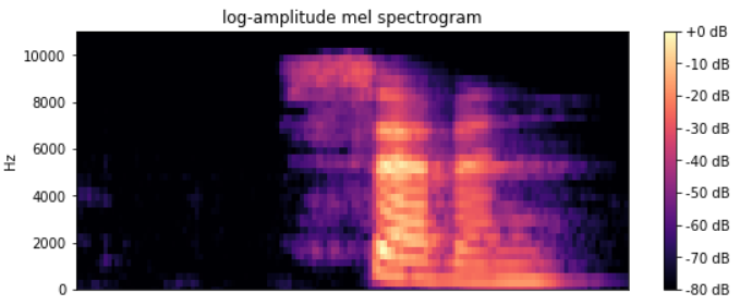
Figure 1. Mel spectrogram of the word ‘seven’

Before you begin

Complete the following steps before starting the tutorial.

Install ELL on your computer (Windows, Ubuntu Linux, macOS).
Follow the instructions for setting up your Raspberry Pi.

What you will need

Laptop or desktop computer
Raspberry Pi 3
USB microphone

Overview

The audio file seven.wav shown in Figure 1 is a mel spectrogram, generated by a mel-frequency cepstrum audio transformer. The horizontal bands correspond to the different frequencies of vocal chords. This frequency map is something that a neural network can learn to recognize through the use of a classifier model. The classifier model file contains a deep neural network trained for keyword spotting on a Kaggle audio dataset, which consists of 60,000 recordings of 30 different keywords. (Keywords that the classifier should recognize are in the categories.txt file and include the following: bed, bird, cat, dog, down, eight, five, four, go, happy, house, left, marvin, nine, no, off, on, one, right, seven, sheila, six, stop, three, tree, two, up, wow, yes, zero.)

In this tutorial, you’ll download a pretrained keyword spotting model from the Embedded Learning Library (ELL) audio gallery to a laptop or desktop computer. You’ll compile the model and wrap it in a Python module. Finally, you’ll write a simple Python script that captures audio from the Raspberry Pi’s microphone and then attempts to detect the keywords spoken.

Activate your environment and create a tutorial directory

After following the setup instructions, you’ll have an Anaconda environment named py36 on your laptop or desktop computer. On your computer, open a terminal window and activate your Anaconda environment.

[Linux/macOS] source activate py36
[Windows] activate py36

Create a directory for this tutorial anywhere on your computer and cd into it.

Download the featurizer model and the classifier model

On your laptop or desktop computer, download this ELL featurizer model file and this ELL classifier model file into your new tutorial directory.

Save the files locally as featurizer.ell.zip and GRU110KeywordSpotter.ell.zip. The 16k suffix is to remind us that these models expect 16 kHz audio input:

curl --location -O https://github.com/Microsoft/ELL-models/raw/master/models/speech_commands_v0.01/BluePaloVerde/featurizer.ell.zip

curl --location -O https://github.com/Microsoft/ELL-models/raw/master/models/speech_commands_v0.01/BluePaloVerde/GRU110KeywordSpotter.ell.zip

Unzip the compressed files and rename them to the shorter names:

Note On Windows computers, the unzip utility is distributed as part of Git. For example, in \Program Files\Git\usr\bin. On Linux computers, you can install unzip using the apt-get install unzip command.

unzip featurizer.ell.zip
unzip GRU110KeywordSpotter.ell.zip
[Linux/macOS] mv GRU110KeywordSpotter.ell classifier.ell
[Windows] ren GRU110KeywordSpotter.ell classifier.ell

Next, download the categories.txt file from here and save it in the directory.

curl --location -o categories.txt https://github.com/microsoft/ELL-models/raw/master/models/speech_commands_v0.01/BluePaloVerde/categories.txt

This file contains the names of the 30 keywords that the model is trained to recognize and one category reserved for background noise. For example, if the model recognizes category 11, you can read line 11 of the categories.txt file to find out that it recognized the word “happy.”

There should now be a featurizer.ell file and a classifier.ell file in your directory.

Compile and run the model on your laptop or desktop computer

Before deploying the model to the Raspberry Pi device, practice deploying it to your laptop or desktop computer. Deploying an ELL model requires two steps. First, you’ll run the wrap tool, which both compiles the featurizer.ell and classifier.ell models into machine code and generates a CMake project to build a Python wrapper for it. Second, you’ll call CMake to build the Python library.

Run wrap as follows, replacing <ELL-root> with the path to the ELL root directory (the directory where you cloned the ELL repository).

python <ELL-root>/tools/wrap/wrap.py --model_file featurizer.ell --target host --outdir compiled_featurizer --module_name mfcc
python <ELL-root>/tools/wrap/wrap.py --model_file classifier.ell --target host --outdir compiled_classifier --module_name model

Here, you used the command line option of --target host, which tells wrap to generate machine code for execution on the laptop or desktop computer, rather than machine code for the Raspberry Pi device. This results in the following output.

compiling model...
generating python interfaces for featurizer in featurizer
running opt...
running llc...
success, now you can build the 'featurizer' folder

Similar output results for the classifier model. The wrap tool creates a CMake project, so you should have two new directories, named compiled_featurizer and compiled_classifier. You can now build these using a build script:

mkdir build
cd build
[Linux/macOS] cmake .. -DCMAKE_BUILD_TYPE=Release && make && cd ../..
[Windows] cmake -G "Visual Studio 16 2019" -A x64 .. && cmake --build . --config Release && cd ..\..

Run this script on both the compiled_featurizer and compiled_classifier folders.

Now, you are almost ready to use these compiled models. Before you do, copy over some Python helper code. This code uses the pyaudio library to read .wav files or to read input from your microphone by converting the raw PCM data into the correct scale of floating point numbers needed for the featurizer model input.

[Linux/macOS] cp <ELL-root>/tools/utilities/pythonlibs/audio/*.py .
[Windows] copy <ELL-root>\tools\utilities\pythonlibs\audio\*.py .

Invoke the model on your computer

The next step is to create a Python script that

Loads the compiled models
Sends audio to the featurizer model
Send the featurizer model output to the classifier model
Interprets the classifier model’s output. (View the full script here.)

Now, one of the audio scripts you just copied is named run_classifier.py and so you will use that here. The inner loop inside that script is transforming the audio using the featurizer and then calling predict as follows:

while True:
    feature_data = transform.read()
    if feature_data is None:
        break
    else:
        prediction, probability, label = predictor.predict(feature_data)
        if probability is not None:
            percent = int(100 * probability)
            print("<<< DETECTED ({}) {}% {} >>>".format(prediction, percent, label))

So try it out using the seven.wav file included with this tutorial. Make a directory named audio and copy the seven.wav file into it. Then run the following:

python run_classifier.py --featurizer compiled_featurizer/mfcc --classifier compiled_classifier/model --categories categories.txt --wav_file audio --sample_rate 16000 --auto_scale

Output similar to this will be displayed:

<<< DETECTED (20) 99% 'seven' >>>
<<< DETECTED (20) 99% 'seven' >>>
<<< DETECTED (20) 99% 'seven' >>>
<<< DETECTED (20) 99% 'seven' >>>
<<< DETECTED (20) 99% 'seven' >>>
<<< DETECTED (20) 99% 'seven' >>>
<<< DETECTED (20) 99% 'seven' >>>
<<< DETECTED (20) 99% 'seven' >>>
Average processing time: 0.00040631294250488277

As the audio is streaming to the classifier, it begins to detect the word. When it passes the confidence threshold of 0.6, it starts printing the results, and you can see that as the word completes the classifier gets more confident, climbing to 99% confidence in this example. The confidence will then drop off as the audio ends because the classifier runs past the end of the word. The average processing time shows how long the feature and classifier models took to execute each frame of audio input in seconds, so the time shown here is half a millisecond, which is not bad, it means these models will be able to easily keep up with real-time audio input.

More about configuration

Use the following tips and information to adjust noise levels, use a USB microphone, and test models.

Modulating output. To experiment with the configuration, set the threshold and smoothing value to zero and see all the output from the classifier. This will make the classifier output more noisy, which is why some smoothing of the output is recommended.
USB microphone. If you have a USB microphone attached to your computer, try running run_classifier.py with no wav_file and it will process your voice input. When you use a microphone you will need to make sure the gain is high. Test your microphone using your favorite voice recorder app, and if the audio recording is nice and loud then it should work well. The classifier was trained on auto-gain leveled input, so if your microphone is too quiet the classifier will not work. Because the microphone input is an infinite stream you will also see a much longer “tail” on the classifier output as it drops back to 60% during the “silence” period between your spoken keywords. Type ‘x’ to terminate the script.
Testing models. Play with the view_audio.py to see a simple GUI app for testing the models. It has the same command line arguments as run_classifier.py and a few more, like --threshold 0.5 and --ignore_label 0 and don’t forget --auto_scale. This app also shows you what your mel spectrograms look like.

Compile the model for execution on the Raspberry Pi device

All the same steps you completed, above, will work on your Raspberry Pi 3 device. The only difference is you call wrap with the command line argument --target pi3. In preparation for this, delete these folders so that the wrap tool can create new folders with Pi 3 code in them.

rm -rf compiled_featurizer
rm -rf compiled_classifier

Then run this:

python <ELL-root>/tools/wrap/wrap.py --model_file featurizer.ell --target pi3 --outdir compiled_compiled_featurizer --module_name mfcc
python <ELL-root>/tools/wrap/wrap.py --model_file classifier.ell --target pi3 --outdir compiled_compiled_classifier --module_name model

You are ready to move to the Raspberry Pi. If your Pi is accessible over the network, copy the directory using the Unix scp tool or the Windows WinSCP tool.

After you copy the entire tutorial folder over to your Raspberry Pi, continue with the build steps you did earlier, only on the Pi this time. Specifically, build the compiled_featurizer and compiled_classifier projects.

Install pyaudio components:

sudo apt-get install python-pyaudio python3-pyaudio portaudio19-dev
pip install pyaudio

Now you can run the run_classifier.py script on the Pi with the same command line arguments you used earlier and see how it does. On the Pi you will see an average processing time of about 2.3 milliseconds, which means real-time audio processing is possible here too.

Next steps

The ELL gallery offers different models for keyword spotting. Some are slow and accurate, while others are faster and less accurate. Different models can even lead to different power draw on the Raspberry Pi. Repeat the steps above with different models.

This tutorial used the wrap tool as a convenient way to compile the model and prepare for building its Python wrapper. To learn more, read the wrap documentation.

Troubleshooting

If you are not getting any results from run_classifier.py or view_audio.py then check the sample_rate information in train_results.json file from the model gallery. If you see a sample rate of 8000 then you need to pass this information to run_classifier.py as the command line argument: --sample_rate 8000. Similarly, check if ‘auto_scale’ was set to true, and if so pass --auto_scale to the python script.

Look for troubleshooting tips at the end of the Raspberry Pi Setup Instructions.