Dataflow Modeling
How Brainsmith systematically bridges the semantic gap between ONNX's model-level abstractions and RTL's cycle-accurate streaming implementation.
Introduction
ONNX describes neural network computation in terms of complete tensors—a LayerNorm operates on an entire (1, 224, 224, 64) activation map. Hardware executes on bit-streams cycling through circuits—16 INT8 elements processed per clock cycle, streamed over hundreds of cycles.
This semantic gap must be bridged systematically. Without a formal model linking tensor operations to streaming execution, you cannot:
- Automatically estimate performance - Calculate cycle counts, throughput, and latency from ONNX graph structure
- Generate infrastructure - Derive FIFO depths, width converters, and buffering requirements from tensor shapes
- Enable design space exploration - Determine valid parallelization ranges and resource tradeoffs without manual analysis
- Compose heterogeneous kernels - Connect elementwise, reduction, and attention operations with different processing patterns
Data Hierarchy: TENSOR/BLOCK/STREAM
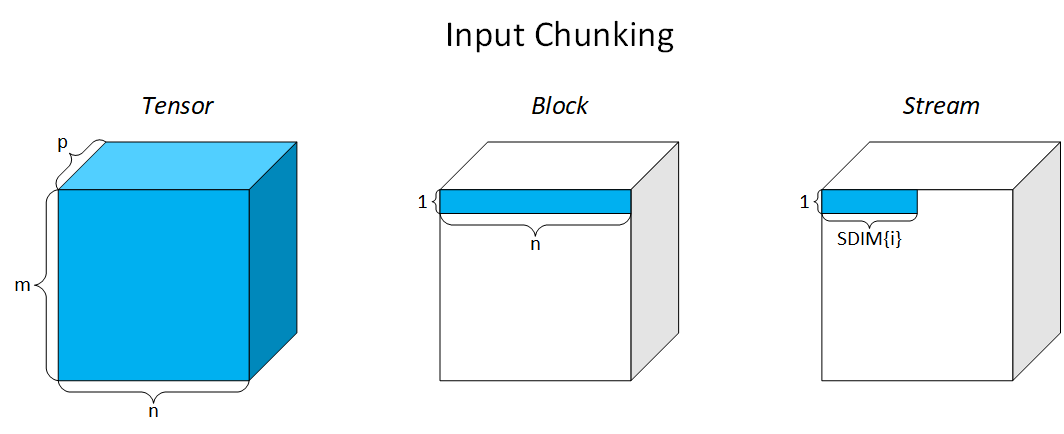
Three Tiers of Refinement
Brainsmith bridges this gap through a three-tier data hierarchy: TENSOR → BLOCK → STREAM. Each tier refines how data is represented and processed:
TENSOR - Complete dimensions from ONNX graph (e.g., (1, 224, 224, 64))
- Defines functional correctness and accuracy requirements
- Extracted from ModelWrapper's tensor shape information
- Represents the semantic unit of computation from the model
BLOCK - Kernel's atomic computation unit (e.g., (1, 7, 7, 64))
- Data required for one cycle of the kernel's computation state
- Controls memory footprint, pipeline depth, and latency
- Defined by
block_tilingtemplate in schema - Determines valid parallelization ranges (STREAM cannot exceed BLOCK)
STREAM - Elements processed per clock cycle (e.g., 16 8-bit Integers)
- Determines throughput and resource usage
- Defined by
stream_tilingtemplate in schema - Constrained by BLOCK shape (cannot exceed block dimensions)
- Resolved during DSE configuration (SIMD, PE parameters)
Kernel-Specific Block Semantics
The BLOCK abstraction level is necessary because some kernels cannot arbitrarily increase parallelism up to the full TENSOR shape. Consider the following examples, and how the BLOCK shape adapts to kernel computation characteristics:
Simple kernels (elementwise operations like Add, Multiply):
- BLOCK = TENSOR (entire input processed as one unit)
- No intermediate computation state between elements
- STREAM parallelization limited only by resource availability
- Example: Add with input
(1, 224, 224, 64)→ BLOCK(1, 224, 224, 64), STREAM(1, 1, 1, 16)
Complex kernels (reduction operations like MatMul, LayerNorm):
- BLOCK = one quantum of the calculation state
- Example: Dot product BLOCK = one input vector
- Kernel must accumulate/reduce across BLOCK before producing output
- STREAM parallelization cannot exceed BLOCK dimensions
- Example: LayerNorm with input
(1, 224, 224, 64)→ BLOCK(1, 1, 1, 64), STREAM(1, 1, 1, 16)
Lowering from ONNX to RTL
The streaming data hierarchy enables automatic derivation of hardware execution characteristics:
# Spatial decomposition
tensor_blocks = ceil(tensor_dim / block_dim)

# Temporal execution
stream_cycles = ceil(block_dim / stream_dim)

# Total latency
total_cycles = prod(tensor_blocks) × prod(stream_cycles)
Example: For tensor (100, 64), block (32, 16), stream (8, 4):
- Tensor blocks:
(4, 4)→ 16 blocks cover the full tensor - Stream cycles:
(4, 4)→ 16 cycles stream each block - Total cycles: 256 (16 blocks × 16 cycles per block)
This calculation forms the basis for: - Performance estimation - Cycle counts and throughput - Resource estimation - Memory requirements from block sizes - DSE constraints - Valid parallelization ranges
Inter-Kernel Dataflow
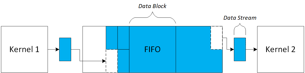
Kernels communicate via streaming interfaces, producing and consuming data cycle-by-cycle. Elastic FIFOs between kernels accumulate these streams as data blocks for buffering, then stream them out to downstream consumers. This infrastructure automatically adapts to different kernel semantics through shape-driven buffering.
Composing Kernels with Different Block Semantics
Consider a simple pipeline: Add → LayerNorm → Softmax
Add (elementwise)           LayerNorm (reduction)       Softmax (reduction)
BLOCK = TENSOR (1,224,64)   BLOCK = (1,1,64)           BLOCK = (1,1,N_classes)
STREAM = (1,1,16)           STREAM = (1,1,16)          STREAM = (1,1,8)
What happens at kernel boundaries:
-
Add → LayerNorm: Producer outputs (1,224,64) blocks, consumer expects (1,1,64) blocks
-
FIFO buffers shape transformation
- Add streams 14 blocks × 16 cycles each = 224 cycles
-
LayerNorm consumes in (1,1,64) chunks, computing normalization per spatial position
-
LayerNorm → Softmax: Block shapes may differ based on computation semantics
-
Each kernel's BLOCK reflects its reduction domain
- FIFOs provide elastic buffering for rate adaptation
Automatic Infrastructure Derivation
Block and stream shapes drive hardware generation:
FIFO Depths - Determined by producer/consumer rate mismatch:
producer_rate = prod(block_shape) / prod(stream_shape)  # cycles per block
consumer_rate = # depends on consumer's internal pipeline depth
fifo_depth = max(producer_burst, consumer_backpressure_tolerance)
Implementation Reality
The formula above describes the theoretical basis for FIFO sizing. In practice, the current implementation uses iterative cycle-accurate RTL simulation to converge on efficient FIFO depths. This will be expanded on in future releases.
Stream Width Matching - Interface widths must align:
- Producer STREAM=(1,1,16) × INT8 → 128-bit AXI-Stream
- Consumer expects matching width or automatic width conversion
- Datatype changes (INT8 → FLOAT32) insert conversion logic
Rate Mismatch Handling - Kernels may have different throughputs:
- Elementwise: 1 output per cycle (after initial latency)
- Reduction: Multiple cycles per output (accumulation phase)
- FIFOs absorb transient rate differences, prevent pipeline stalls
Schema-Driven Interface Resolution
Schemas declare interfaces using templates that adapt to runtime shapes:
# Producer (Add kernel)
OutputSchema(
    block_tiling=[FULL_DIM, FULL_DIM, FULL_DIM],  # Process entire spatial dims
    stream_tiling=[1, 1, "PE"]                      # Parallelize over channels
)

# Consumer (LayerNorm kernel)
InputSchema(
    block_tiling=[FULL_DIM, FULL_DIM, FULL_DIM],  # Same spatial processing
    stream_tiling=[1, 1, "SIMD"]                    # Match channel parallelism
)
At compile time:
- ONNX tensor shapes resolve
FULL_DIM→ actual dimensions - DSE parameters (PE=16, SIMD=16) resolve stream tiling
- Infrastructure generates FIFOs matching computed shapes
- Validation ensures producer/consumer compatibility
This declarative approach separates what (tensor semantics) from how (hardware implementation), enabling design space exploration while maintaining correctness by construction. The compiler automatically inserts width converters, reshaping logic, and elastic buffering as needed.
Design Space Implications
The dataflow modeling hierarchy directly constrains design space exploration:
Valid Parallelization Ranges:
- STREAM dimensions must be divisors of BLOCK dimensions
- For BLOCK=(64,), valid STREAM values are {1, 2, 4, 8, 16, 32, 64}
- Invalid: STREAM=128 (exceeds block size)
Performance vs Resource Tradeoffs:
- Increasing STREAM → Higher throughput, more DSP/LUT usage
- Increasing BLOCK → More on-chip memory, potentially higher latency
- Heterogeneous pipelines: Balance per-kernel parallelization against total resource budget
Configuration Constraints:
- Producer/consumer STREAM widths must match (or have automatic conversion)
- Total pipeline throughput limited by slowest kernel
- FIFO depths must accommodate worst-case rate mismatches