import graspologic

import numpy as np
import matplotlib.pyplot as plt

Padded Graph Matching

Consider the scenario where one would like to match graphs \(A\) and \(B\) with \(n_1\) and \(n_2\) nodes, respectively, where \(n_1 < n_2\). The most straightforward fashion to ‘pad’ \(A\), such that \(A\) and \(B\) have the same shape, is to add \(n_2 - n_1\) isolated nodes to \(A\) (represented as empty row/columns in the adjacency matrix). This padding scheme is known as \(\textit{naive padding}\), substituting \(A \oplus 0_{(n_2-n_1)x(n_2-n_1)}\) and \(B\) in place of \(A\) and \(B\), respectively.

The effect of this is that one matches \(A\) to the best subgraph of \(B\). That is, the isolated vertices added to \(A\) through padding have an affinity to the low-density subgraphs of \(B\), in effect giving the isolates a false signal.

Instead, we may desire to match \(A\) to the best fitting induced subgraph of \(B\). This padding scheme is known as \(\textit{adopted padding}\), and is achieved by substituting \(\tilde{A} \oplus 0_{(n_2-n_1)x(n_2-n_1)}\) and \(\tilde{B}\) in place of \(A\) and \(B\), respectively, where \(\tilde{A} = 2A - 1_{n_1}1_{n_1}^T\) and \(\tilde{B} = 2B - 1_{n_2}1_{n_2}^T\).

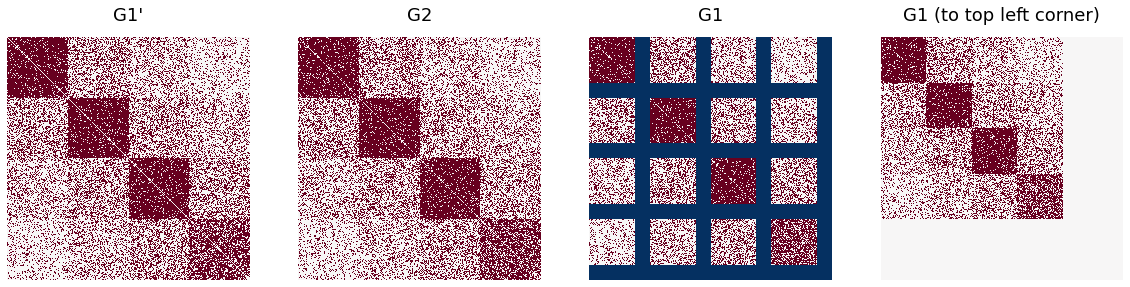
To demonstrate the difference between the two padding schemes, we sample two graph’s \(G_1'\) and \(G_2\), each having 400 vertices, from a \(0.5 \sim SBM(4,b,\Lambda)\), where b assigns 100 vertices to each of the k = 4 blocks, and

\begin{align*} \Lambda &= \begin{bmatrix} 0.9 & 0.4 & 0.3 & 0.2\\ 0.4 & 0.9 & 0.4 & 0.3\\ 0.3 & 0.4 & 0.9 & 0.4\\ 0.2 & 0.3 & 0.4 & 0.7 \end{bmatrix}\\ \end{align*}

We realize \(G_1\) from \(G_1'\) by removing 25 nodes from each block of \(G_1'\), yielding a 300 node graph (example adapted from section 2.5 of [1]).

The goal of the matching in this case is to recover \(G_1\) by matching the right most figure below and \(G_2\). That is, we seek to recover the shared community structure common between two graphs of differing shapes.

[1] D. Fishkind, S. Adali, H. Patsolic, L. Meng, D. Singh, V. Lyzinski, C. Priebe, “Seeded graph matching”, Pattern Recognit. 87 (2019) 203–215

SBM correlated graph pairs

# simulating G1', G2, deleting 25 vertices
from graspologic.match import GraphMatch as GMP
from graspologic.simulations import sbm_corr
from graspologic.plot import heatmap
np.random.seed(1)

directed = False
loops = False
block_probs = [[0.9,0.4,0.3,0.2],
                [0.4,0.9,0.4,0.3],
                [0.3,0.4,0.9,0.4],
                [0.2,0.3,0.4,0.7]]
n =100
n_blocks = 4
rho = 0.5
block_members = np.array(n_blocks * [n])
n_verts = block_members.sum()
G1p, G2 = sbm_corr(block_members,block_probs, rho, directed, loops)
G1 = np.zeros((300,300))
c = np.copy(G1p)

step1 = np.arange(4) * 100 + 75
step2 = np.arange(5) * 75
step3 = np.arange(4) * 100
for i in range(len(step1)):
    block1 = np.arange(step1[i], step1[i]+25)
    c[block1,:] = -1
    c[:, block1] = -1
    for j in range(len(step3)):
        G1[step2[i]:step2[i+1], step2[j]:step2[j+1]] = G1p[step3[i]: step1[i], step3[j]:step1[j]]

topleft_G1 = np.zeros((400,400))
topleft_G1[:300,:300] = G1
fig, axs = plt.subplots(1, 4, figsize=(20, 10))
heatmap(G1p, ax=axs[0], cbar=False, title="G1'")
heatmap(G2, ax=axs[1], cbar=False, title="G2")
heatmap(c, ax=axs[2], cbar=False, title="G1")
_ = heatmap(topleft_G1, ax=axs[3], cbar=False, title="G1 (to top left corner)")

Naive vs Adopted Padding

np.random.seed(1)

gmp_naive = GMP(padding='naive')
seed1 = np.random.choice(np.arange(300),8)
seed2 = [int(x/75)*25 + x for x in seed1]
gmp_naive = gmp_naive.fit(G2, G1, seed2, seed1)
G1_naive = topleft_G1[gmp_naive.perm_inds_][:, gmp_naive.perm_inds_]

gmp_adopted = GMP(padding='adopted')
gmp_adopted = gmp_adopted.fit(G2, G1, seed2, seed1)
G1_adopted = topleft_G1[gmp_adopted.perm_inds_][:, gmp_adopted.perm_inds_]

fig, axs = plt.subplots(1, 2, figsize=(14, 7))
heatmap(G1_naive, ax=axs[0], cbar=False, title="Naive Padding")
heatmap(G1_adopted, ax=axs[1], cbar=False, title="Adopted Padding")

naive_matching = np.concatenate([gmp_naive.perm_inds_[x * 100 : (x * 100) + 75] for x in range(n_blocks)])
adopted_matching = np.concatenate([gmp_adopted.perm_inds_[x * 100 : (x * 100) + 75] for x in range(n_blocks)])

print(f'Match ratio of nodes remaining in G1, with naive padding: {sum(naive_matching == np.arange(300))/300}')
print(f'Match ratio of nodes remaining in G1, with adopted padding: {sum(adopted_matching == np.arange(300))/300}')

Match ratio of nodes remaining in G1, with naive padding: 0.15333333333333332
Match ratio of nodes remaining in G1, with adopted padding: 1.0

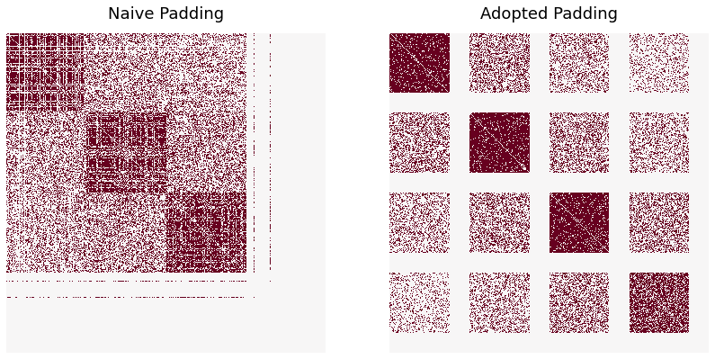
We observe that the two padding schemes perform as expected. The naive scheme permutes \(G_1\) such that it matches a subgraph of \(G_2\), specifically the subgraph of the first three blocks. Additionally, (almost) all isolated vertices of \(G_1\) are permuted to the fourth block of \(G_2\).

On the other hand, we see that adopted padding preserves the common block structure between \(G_1\) and \(G_2\).