Seeded Graph Matching (SGM)

import numpy as np
import matplotlib.pyplot as plt
import seaborn as sns
import random
np.random.seed(8888)

Seeded Graph Matching (SGM) is a version of the graph matching problem where one is first given a partial alignment of the nodes. This algorithm is an modification of the Fast Approximate QAP (FAQ) algorithm (Vogelstein, 2015), as described in Seeded graph matching (Fishkind, 2018). For a more in depth explanation of the graph matching problem and FAQ, view the FAQ tutorial.

from graspologic.match import GraphMatch as GMP
from graspologic.plot import heatmap
from graspologic.simulations import er_corr, sbm, sbm_corr

SGM on Correlated Graph Pairs

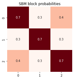
To demonstrate the effectiveness of SGM, the algorithm will be applied on a pair of correlated SBM graphs (undirected, no self loops) \(G_1, G_2 \sim SBM\,(n, p, rho)\) with the following parameters: \begin{align*} n &= [100, 100, 100]\\ p &= \begin{bmatrix} 0.7 & 0.3 & 0.4\\ 0.3 & 0.7 & 0.3\\ 0.4 & 0.3 & 0.7 \end{bmatrix}\\ rho &= 0.9 \end{align*}

directed = False
loops = False
n_per_block = 75
n_blocks = 3
block_members = np.array(n_blocks * [n_per_block])
n_verts = block_members.sum()
rho = .9
block_probs = np.array([[0.7, 0.3, 0.4], [0.3, 0.7, 0.3], [0.4, 0.3, 0.7]])
fig, ax = plt.subplots(1, 1, figsize=(4, 4))
sns.heatmap(block_probs, cbar=False, annot=True, square=True, cmap="Reds", ax=ax)
ax.set_title("SBM block probabilities")

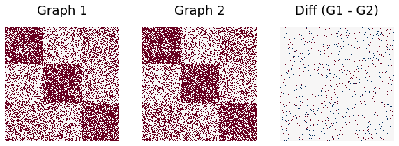
A1, A2 = sbm_corr(block_members, block_probs, rho, directed=directed, loops=loops)
fig, axs = plt.subplots(1, 3, figsize=(10, 5))
heatmap(A1, ax=axs[0], cbar=False, title="Graph 1")
heatmap(A2, ax=axs[1], cbar=False, title="Graph 2")
_ = heatmap(A1 - A2, ax=axs[2], cbar=False, title="Diff (G1 - G2)")

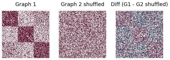
To demonstrate the effectiveness of SGM, as well as why having seeds is important, we will randomly shuffle the vertices of Graph 2. This random permutation is stored, and unshuffled, such that we have available the optimal permutation that returns the original graph 2.

Shuffling graph 2

Here we see that after shuffling graph 2, there are many more edge disagreements, as expected.

node_shuffle_input = np.random.permutation(n_verts)
A2_shuffle = A2[np.ix_(node_shuffle_input, node_shuffle_input)]
node_unshuffle_input = np.array(range(n_verts))
node_unshuffle_input[node_shuffle_input] = np.array(range(n_verts))

fig, axs = plt.subplots(1, 3, figsize=(10, 5))
heatmap(A1, ax=axs[0], cbar=False, title="Graph 1")
heatmap(A2_shuffle, ax=axs[1], cbar=False, title="Graph 2 shuffled")
_ = heatmap(A1 - A2_shuffle, ax=axs[2], cbar=False, title="Diff (G1 - G2 shuffled)")

Unshuffling graph 2 without seeds

First, we will run SGM on graph 1 and the shuffled graph 2 with no seeds, and return the match ratio, that is the fraction of vertices that have been correctly matched.

sgm = GMP()
sgm = sgm.fit(A1,A2_shuffle)
A2_unshuffle = A2_shuffle[np.ix_(sgm.perm_inds_, sgm.perm_inds_)]

fig, axs = plt.subplots(1, 3, figsize=(10, 5))
heatmap(A1, ax=axs[0], cbar=False, title="Graph 1")
heatmap(A2_unshuffle, ax=axs[1], cbar=False, title="Graph 2 unshuffled")
heatmap(A1 - A2_unshuffle, ax=axs[2], cbar=False, title="Diff (G1 - G2 unshuffled)")

match_ratio = 1-(np.count_nonzero(abs(sgm.perm_inds_-node_unshuffle_input))/n_verts)
print("Match Ratio with no seeds: ", match_ratio)

Match Ratio with no seeds:  0.008888888888888835

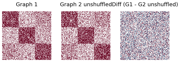
While the predicted permutation for graph 2 did recover the basic structure of the stochastic block model (i.e. graph 1 and graph 2 look qualitatively similar), we see that the number of edge disagreements between them is still quite high, and the match ratio quite low.

Unshuffling graph 2 with 10 seeds

Next, we will run SGM with 10 seeds randomly selected from the optimal permutation vector found ealier. Although 10 seeds is only about 4% of the 300 node graph, we will observe below how much more accurate the matching will be compared to having no seeds.

W1 = np.sort(random.sample(list(range(n_verts)),10))
W1 = W1.astype(int)
W2 = np.array(node_unshuffle_input[W1])

sgm = GMP()
sgm = sgm.fit(A1,A2_shuffle,W1,W2)
A2_unshuffle = A2_shuffle[np.ix_(sgm.perm_inds_, sgm.perm_inds_)]

fig, axs = plt.subplots(1, 3, figsize=(10, 5))
heatmap(A1, ax=axs[0], cbar=False, title="Graph 1")
heatmap(A2_unshuffle, ax=axs[1], cbar=False, title="Graph 2 unshuffled")
heatmap(A1 - A2_unshuffle, ax=axs[2], cbar=False, title="Diff (G1 - G2 unshuffled)")

match_ratio = 1-(np.count_nonzero(abs(sgm.perm_inds_-node_unshuffle_input))/n_verts)
print("Match Ratio with 10 seeds: ", match_ratio)

Match Ratio with 10 seeds:  1.0

From the results above, we see that when running SGM on the same two graphs, with no seeds there is match ratio is quite low. However including 10 seeds increases the match ratio to 100% (meaning that the shuffled graph 2 was completely correctly unshuffled).