Stochastic Block Model (SBM)

import graspologic

import matplotlib.pyplot as plt
import numpy as np
%matplotlib inline

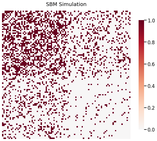
Unlike Erdos-Renyi (ER) models, a Stochastic Block Model (SBM) produces graphs containing communities: disjoint subgraphs characterized by differing edge probabilities for vertices within and between communities (1).

SBM is parametrized by the number of vertices in each community \(n\), and a block probability matrix \(P \in \mathbb{R}^{n x n}\) where each element specifies the probability of an edge in a particular block. One can think of SBM as a collection of ER graphs where each block corresponds to an ER graph.

Below, we sample a two-block SBM (undirected, no self-loops) with following parameters:

\begin{align*} n &= [50, 50]\\ P &= \begin{bmatrix} 0.5 & 0.2\\ 0.2 & 0.05 \end{bmatrix} \end{align*}

The diagonals correspond to probability of an edge within blocks and the off-diagonals correspond to probability of an edge between blocks.

from graspologic.simulations import sbm

n = [50, 50]
p = [[0.5, 0.2],
     [0.2, 0.05]]

np.random.seed(1)
G = sbm(n=n, p=p)

Visualize the graph using heatmap

from graspologic.plot import heatmap

_ = heatmap(G, title ='SBM Simulation')

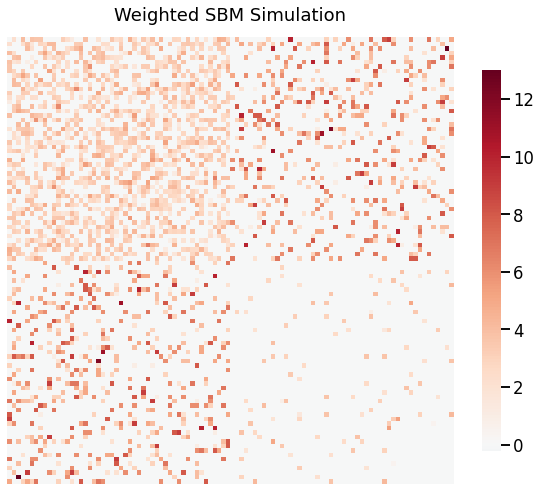
Weighted SBM Graphs

Similar to ER simulations, sbm() functions provide ways to sample weights for all edges that were sampled via a probability distribution function. In order to sample with weights, you can either:

1. Provide a single probability distribution function with corresponding keyword arguments for the distribution function. All weights will be sampled using the same function.

2. Provide a probability distribution function with corresponding keyword arguments for each block.

Below we sample a SBM (undirected, no self-loops) with the following parameters:

\begin{align*} n &= [50, 50]\\ P &= \begin{bmatrix}0.5 & 0.2\\ 0.2 & 0.05 \end{bmatrix} \end{align*}

and the weights are sampled from the following probability functions:

\begin{align*} PDFs &= \begin{bmatrix}Normal & Poisson\\ Poisson & Normal \end{bmatrix}\\ Parameters &= \begin{bmatrix}{\mu=3, \sigma^2=1} & {\lambda=5}\\ {\lambda=5} & {\mu=3, \sigma^2=1} \end{bmatrix} \end{align*}

from numpy.random import normal, poisson

n = [50, 50]
p = [[0.5, 0.2],
     [0.2, 0.05]]
wt = [[normal, poisson],
      [poisson, normal]]
wtargs = [[dict(loc=3, scale=1), dict(lam=5)],
          [dict(lam=5), dict(loc=3, scale=1)]]

G = sbm(n=n, p=p, wt=wt, wtargs=wtargs)

Visualize the graph using heatmap

_ = heatmap(G, title='Weighted SBM Simulation')