High-Level Analysis
vignette.RmdSome common parameters
set.seed(1337)
N = 1000
K = 3
err_sd = 1
Simple Example
Let’s get some fake data
X = matrix(runif(N*K), ncol=K) #Features for splitting partition
d = rbinom(N, 1, 0.5) #treatment assignment
tau = as.integer(X[,1]>.5)*2-1 #true treatment effect (just heterogeneous across X1)
y = d*tau + rnorm(N, 0, err_sd) #outcome
est_part0 = fit_estimate_partition(y, X, d, cv_folds=2)
get_desc_df(est_part0)
#>            X1 N_est param_ests         pval
#> 1 <=0.5050542   261 -0.7767593 3.681519e-09
#> 2  >0.5050542   239  0.8697289 3.792252e-11
We typically want a high-level partition for “human” consumption. To save time, avoid cells with too few observations, and reduce the chance of splitting from running many noisy tests, it’s common to only look for a few splits per dimension. If we don’t specify this, the function will try every possible split across each dimension.
# With just a scalar, we will split at points equal across the quantile-distribution for each feature.
breaks = 5
#Otherwise we can explicitly list the potential splits to evaluate.
breaks = rep(list(seq(breaks)/(breaks+1)), K)
est_part = fit_estimate_partition(y, X, d, breaks_per_dim=breaks, cv_folds=2)
plot(est_part)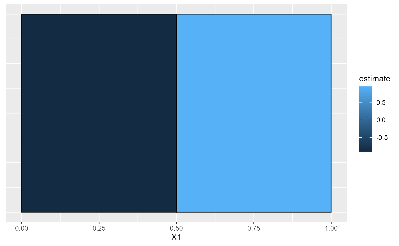
get_desc_df(est_part)
#>      X1 N_est param_ests         pval
#> 1 <=0.5   255 -0.9035292 3.379837e-12
#> 2  >0.5   245  0.9557823 2.823001e-12
We can manually estimate this simple model given the partition
est_df = data.frame(y=y, d=d, f=predict(est_part$partition, X))
summary(lm(y~0+f+d:f, data=est_df[-est_part$index_tr,]))
#>
#> Call:
#> lm(formula = y ~ 0 + f + d:f, data = est_df[-est_part$index_tr,
#>     ])
#>
#> Residuals:
#>     Min      1Q  Median      3Q     Max
#> -3.1360 -0.6908 -0.0019  0.7014  2.6253
#>
#> Coefficients:
#>                               Estimate Std. Error t value Pr(>|t|)
#> f(-1,0.5].(-0.999,2].(-1,2]   -0.09209    0.08434  -1.092    0.275
#> f(0.5,2].(-0.999,2].(-1,2]     0.05627    0.08786   0.640    0.522
#> f(-1,0.5].(-0.999,2].(-1,2]:d -0.90353    0.12559  -7.194 2.33e-12 ***
#> f(0.5,2].(-0.999,2].(-1,2]:d   0.95578    0.12769   7.485 3.28e-13 ***
#> ---
#> Signif. codes:  0 '***' 0.001 '**' 0.01 '*' 0.05 '.' 0.1 ' ' 1
#>
#> Residual standard error: 0.9979 on 496 degrees of freedom
#> Multiple R-squared:  0.3218, Adjusted R-squared:  0.3164
#> F-statistic: 58.85 on 4 and 496 DF,  p-value: < 2.2e-16
Sometimes we want a different level of complexity than that picked by CV. Either we can pre-specify which partition in the sequence that we want (using the partition_i parameter), or we can look at the sequence of objective function values and see where additional splits only provide marginal improvements.
print(paste("In-sample Objective function values: ", paste(est_part$is_obj_val_seq, collapse=" ")))
#> [1] "In-sample Objective function values:  -0.00130792756957961 -0.860071145786862 -0.906298192191155 -0.974137597678458 -1.01692472825141 -1.05861007636975 -1.1137648149499 -1.16690858898675 -1.22036187891834 -1.23615779557238"
Compare this with the average treatment effect for the whole and estimation-only samples
est_part$full_stat_df
#>      sample N_est param_ests    var_ests    tstats      ci_u       ci_l
#> N_tr    all  1000 0.03338318 0.005710407 0.4417680 0.1816721 -0.1149057
#> N_es    est   500 0.03350558 0.011765447 0.3088965 0.2466182 -0.1796070
#>           pval
#> N_tr 0.6587528
#> N_es 0.7575295
How important are each of the dimensions of X for the objective function? We refit the model without each dimension and see the change in the objective function
est_part$importance_weights
#> NULL
The first feature is the only one that is useful.
Are there any interactions between the importances? (That is if we remove X1, does the importance of X2 change? This is done by dropping pairs of featurs at a time and see how they differ from single-feature droppings)
est_part$interaction_weights
#> NULL
Essentially no.
Get the observation-level estimated treatment effects.
tau_hat = predict(est_part, new_X=X)With many estimates, we may wish to account for multiple testing when checking if “there are any negative (or positive) effects”
any_neg = test_any_sign_effect(est_part, check_negative=T)
print(paste("Adjusted 1-side p-values testing if negative:", paste(any_neg$pval1s_fdr, collapse=", ")))
#> [1] "Adjusted 1-side p-values testing if negative: 3.37983707236465e-12, 0.999999999998588"
Now let’s look at a case where there’s hereogeneity across all three dimensions.
tau_3 = (as.integer(X[,1]>0.5)*2-1) + (as.integer(X[,2]>0.5)*2-1)*2 + (as.integer(X[,3]>0.5)*2-1)*3
y_3 = d*tau_3 + rnorm(N, 0, err_sd)
est_part_3 = fit_estimate_partition(y_3, X, d, breaks_per_dim=5, partition_i=4)
get_desc_df(est_part_3)
#>            X1          X2          X3 N_est param_ests         pval
#> 1 <=0.4844432 <=0.5158526 <=0.4956977    57 -6.0701075 2.650172e-30
#> 2  >0.4844432 <=0.5158526 <=0.4956977    59 -3.7226053 4.028245e-16
#> 3 <=0.4844432  >0.5158526 <=0.4956977    64 -1.9451039 1.181403e-10
#> 4  >0.4844432  >0.5158526 <=0.4956977    64  0.1690431 5.336151e-01
#> 5 <=0.4844432 <=0.5158526  >0.4956977    63 -0.6908844 3.478647e-02
#> 6  >0.4844432 <=0.5158526  >0.4956977    53  2.3977563 6.423076e-09
#> 7 <=0.4844432  >0.5158526  >0.4956977    72  3.8194994 1.243479e-24
#> 8  >0.4844432  >0.5158526  >0.4956977    68  6.1846918 6.820379e-36
One benefit of grid-based partitions is that you can view easily view 2D slices of full heterogeneity space.
plts = plot(est_part_3)

grid.arrange(plts[[1]], plts[[2]], ncol=2)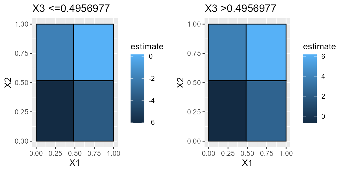
Improving the partition
We can improve the partition by controlling for X’s (either local-linearly or global-flexibly) and using bootstrap “bumping”
est_part_l = fit_estimate_partition(y, X, d, breaks_per_dim=5, ctrl_method = "LassoCV", bump_samples = 20, partition_i=2)LassoCV is a local-linear approach and we can use the global-flexible approach by setting ctrl_method="RF" for a random forest.
Parallel-processing
Parallel-processing the outer-loops
#library(parallel)
#cl <- makeCluster(getOption("cl.cores", default=3)) #see also detectCores()
#fit_res = fit_estimate_partition(..., pr_cl=cl)
#stopCluster(cl)
Multiple core estimates
We can generate a single partition that works across multiple core estimates. We have three options.
- Multiple outcomes, but same sample (single treatment)
tau2 = as.integer(X[,2]>0.5)*2-1
y2_yM = d*tau2 + rnorm(N, 0, err_sd)
y_yM = cbind(y, y2_yM)
est_part_yM = fit_estimate_partition(y_yM, X, d, breaks_per_dim=5, partition_i = 3)
get_desc_df(est_part_yM)
#>            X1          X2 N_est1 N_est2 param_ests1 param_ests2        pval1
#> 1 <=0.4844432 <=0.5158526    130    130  -0.8150777  -1.0797322 1.661861e-05
#> 2  >0.4844432 <=0.5158526    118    118   0.7621012  -1.1433613 7.692081e-06
#> 3 <=0.4844432  >0.5158526    119    119  -1.0825123   0.9278330 1.023561e-08
#> 4  >0.4844432  >0.5158526    133    133   1.0348422   0.6970603 2.502101e-09
#>          pval2
#> 1 9.023729e-10
#> 2 2.241744e-07
#> 3 6.075092e-06
#> 4 1.456469e-04- Multiple treatments, but same sample (single outcome)
d2 = rbinom(N, 1, 0.5)
d_dM = cbind(d, d2)
y_dM =  d*tau + d2*tau2 + rnorm(N, 0, err_sd)
est_part_dM = fit_estimate_partition(y_dM, X, d_dM, breaks_per_dim=5, partition_i = 3)
get_desc_df(est_part_dM)
#>            X1          X2 N_est1 N_est2 param_ests1 param_ests2        pval1
#> 1 <=0.4844432 <=0.5158526    135    135  -0.9762579  -0.9840951 7.622683e-08
#> 2  >0.4844432 <=0.5158526    118    118   0.9325741  -0.7867792 5.249161e-06
#> 3 <=0.4844432  >0.5158526    116    116  -1.2541714   0.7402976 1.460617e-09
#> 4  >0.4844432  >0.5158526    131    131   1.1479998   0.8282607 1.158216e-08
#>          pval2
#> 1 5.822138e-08
#> 2 7.690174e-05
#> 3 1.333272e-04
#> 4 2.509196e-05- Multiple separate samples, each having a single outcome and treatment
y2_MM = d2*tau2 + rnorm(N, 0, err_sd)
y_MM = list(y, y2_MM)
d_MM = list(d, d2)
X_MM = list(X, X)
est_part_MM = fit_estimate_partition(y_MM, X_MM, d_MM, breaks_per_dim=5, partition_i = 3)
get_desc_df(est_part_MM)
#>            X1          X2 N_est1 N_est2 param_ests1 param_ests2        pval1
#> 1 <=0.4844432 <=0.5158526    130    124  -0.9043386  -0.8583915 6.680335e-06
#> 2  >0.4844432 <=0.5158526    122    126   0.7282198  -1.1698914 1.392059e-05
#> 3 <=0.4844432  >0.5158526    128    131  -1.0385968   1.4084632 3.053106e-09
#> 4  >0.4844432  >0.5158526    120    119   1.0489269   0.9796365 8.551001e-08
#>          pval2
#> 1 2.926864e-06
#> 2 2.092628e-08
#> 3 3.320067e-12
#> 4 2.845363e-06
Mean-outcome prediction
alpha = as.integer(X[,1]>0.5)*2-1 #true average outcome effect (just heterogeneous across X1)
y_y = alpha + rnorm(N, 0, err_sd) #outcome
est_part_y = fit_estimate_partition(y_y, X, breaks_per_dim=5, partition_i=2)
get_desc_df(est_part_y)
#>            X1 N_est param_ests         pval
#> 1 <=0.4844432   247 -1.0304578 5.228963e-43
#> 2  >0.4844432   253  0.9447789 5.803037e-32