Recipe: Azure AI Services - Multivariate Anomaly Detection
This recipe shows how you can use SynapseML and Azure AI services on Apache Spark for multivariate anomaly detection. Multivariate anomaly detection allows for the detection of anomalies among many variables or time series, taking into account all the inter-correlations and dependencies between the different variables. In this scenario, we use SynapseML to train a model for multivariate anomaly detection using the Azure AI services, and we then use to the model to infer multivariate anomalies within a dataset containing synthetic measurements from three IoT sensors.
To learn more about the Azure AI Anomaly Detector, refer to this documentation page.
Important
Starting on the 20th of September, 2023 you won’t be able to create new Anomaly Detector resources. The Anomaly Detector service is being retired on the 1st of October, 2026.
Setup
Create an Anomaly Detector resource
Follow the instructions to create an Anomaly Detector resource using the Azure portal or alternatively, you can also use the Azure CLI to create this resource.
- In the Azure portal, select Create in your resource group, and then type Anomaly Detector. Select the Anomaly Detector resource.
- Give the resource a name, and ideally use the same region as the rest of your resource group. Use the default options for the rest, and then select Review + Create and then Create.
- Once the Anomaly Detector resource is created, open it and select the
Keys and Endpointspanel in the left nav. Copy the key for the Anomaly Detector resource into theANOMALY_API_KEYenvironment variable, or store it in theanomalyKeyvariable.
Create a Storage Account resource
In order to save intermediate data, you need to create an Azure Blob Storage Account. Within that storage account, create a container for storing the intermediate data. Make note of the container name, and copy the connection string to that container. You need it later to populate the containerName variable and the BLOB_CONNECTION_STRING environment variable.
Enter your service keys
Let's start by setting up the environment variables for our service keys. The next cell sets the ANOMALY_API_KEY and the BLOB_CONNECTION_STRING environment variables based on the values stored in our Azure Key Vault. If you're running this tutorial in your own environment, make sure you set these environment variables before you proceed.
Now, lets read the ANOMALY_API_KEY and BLOB_CONNECTION_STRING environment variables and set the containerName and location variables.
from synapse.ml.core.platform import find_secret

# An Anomaly Dectector subscription key
anomalyKey = find_secret(
    secret_name="anomaly-api-key", keyvault="mmlspark-build-keys"
)  # use your own anomaly api key
# Your storage account name
storageName = "anomalydetectiontest"  # use your own storage account name
# A connection string to your blob storage account
storageKey = find_secret(
    secret_name="madtest-storage-key", keyvault="mmlspark-build-keys"
)  # use your own storage key
# A place to save intermediate MVAD results
intermediateSaveDir = (
    "wasbs://madtest@anomalydetectiontest.blob.core.windows.net/intermediateData"
)
# The location of the anomaly detector resource that you created
location = "westus2"
First we connect to our storage account so that anomaly detector can save intermediate results there:
spark.sparkContext._jsc.hadoopConfiguration().set(
    f"fs.azure.account.key.{storageName}.blob.core.windows.net", storageKey
)
Let's import all the necessary modules.
import numpy as np
import pandas as pd

import pyspark
from pyspark.sql.functions import col
from pyspark.sql.functions import lit
from pyspark.sql.types import DoubleType
import matplotlib.pyplot as plt

import synapse.ml
from synapse.ml.services.anomaly import *
Now, let's read our sample data into a Spark DataFrame.
df = (
    spark.read.format("csv")
    .option("header", "true")
    .load("wasbs://publicwasb@mmlspark.blob.core.windows.net/MVAD/sample.csv")
)

df = (
    df.withColumn("sensor_1", col("sensor_1").cast(DoubleType()))
    .withColumn("sensor_2", col("sensor_2").cast(DoubleType()))
    .withColumn("sensor_3", col("sensor_3").cast(DoubleType()))
)

# Let's inspect the dataframe:
df.show(5)
We can now create an estimator object, which is used to train our model. We specify the start and end times for the training data. We also specify the input columns to use, and the name of the column that contains the timestamps. Finally, we specify the number of data points to use in the anomaly detection sliding window, and we set the connection string to the Azure Blob Storage Account.
trainingStartTime = "2020-06-01T12:00:00Z"
trainingEndTime = "2020-07-02T17:55:00Z"
timestampColumn = "timestamp"
inputColumns = ["sensor_1", "sensor_2", "sensor_3"]

estimator = (
    SimpleFitMultivariateAnomaly()
    .setSubscriptionKey(anomalyKey)
    .setLocation(location)
    .setStartTime(trainingStartTime)
    .setEndTime(trainingEndTime)
    .setIntermediateSaveDir(intermediateSaveDir)
    .setTimestampCol(timestampColumn)
    .setInputCols(inputColumns)
    .setSlidingWindow(200)
)
Now that we created the estimator, let's fit it to the data:
model = estimator.fit(df)
Once the training is done, we can now use the model for inference. The code in the next cell specifies the start and end times for the data we would like to detect the anomalies in.
inferenceStartTime = "2020-07-02T18:00:00Z"
inferenceEndTime = "2020-07-06T05:15:00Z"

result = (
    model.setStartTime(inferenceStartTime)
    .setEndTime(inferenceEndTime)
    .setOutputCol("results")
    .setErrorCol("errors")
    .setInputCols(inputColumns)
    .setTimestampCol(timestampColumn)
    .transform(df)
)

result.show(5)
When we called .show(5) in the previous cell, it showed us the first five rows in the dataframe. The results were all null because they weren't inside the inference window.
To show the results only for the inferred data, lets select the columns we need. We can then order the rows in the dataframe by ascending order, and filter the result to only show the rows that are in the range of the inference window. In our case inferenceEndTime is the same as the last row in the dataframe, so can ignore that.
Finally, to be able to better plot the results, lets convert the Spark dataframe to a Pandas dataframe.
rdf = (
    result.select(
        "timestamp",
        *inputColumns,
        "results.interpretation",
        "isAnomaly",
        "results.severity"
    )
    .orderBy("timestamp", ascending=True)
    .filter(col("timestamp") >= lit(inferenceStartTime))
    .toPandas()
)

rdf
Format the contributors column that stores the contribution score from each sensor to the detected anomalies. The next cell formats this data, and splits the contribution score of each sensor into its own column.
For Spark3.3 and below versions, the output of select statements will be in the format of List<Rows>, so to format the data into dictionary and generate the values when interpretation is empty, please use the below parse method:
def parse(x):
    if len(x) > 0:
        return dict([item[:2] for item in x])
    else:
        return {"sensor_1": 0, "sensor_2": 0, "sensor_3": 0}
Staring with Spark3.4, the output of the select statement is already formatted as a numpy.ndarry<dictionary> and no need to format the data again, so please use below parse method to generate the values when interpretation is empty:
def parse(x):
    if len(x) == 0:
        return {"sensor_1": 0, "sensor_2": 0, "sensor_3": 0}


rdf["contributors"] = rdf["interpretation"].apply(parse)
rdf = pd.concat(
    [
        rdf.drop(["contributors"], axis=1),
        pd.json_normalize(rdf["contributors"]).rename(
            columns={
                "sensor_1": "series_1",
                "sensor_2": "series_2",
                "sensor_3": "series_3",
            }
        ),
    ],
    axis=1,
)
rdf
Great! We now have the contribution scores of sensors 1, 2, and 3 in the series_0, series_1, and series_2 columns respectively.
Run the next cell to plot the results. The minSeverity parameter specifies the minimum severity of the anomalies to be plotted.
minSeverity = 0.1


####### Main Figure #######
plt.figure(figsize=(23, 8))
plt.plot(
    rdf["timestamp"],
    rdf["sensor_1"],
    color="tab:orange",
    line,
    linewidth=2,
    label="sensor_1",
)
plt.plot(
    rdf["timestamp"],
    rdf["sensor_2"],
    color="tab:green",
    line,
    linewidth=2,
    label="sensor_2",
)
plt.plot(
    rdf["timestamp"],
    rdf["sensor_3"],
    color="tab:blue",
    line,
    linewidth=2,
    label="sensor_3",
)
plt.grid(axis="y")
plt.tick_params(axis="x", which="both", bottom=False, labelbottom=False)
plt.legend()

anoms = list(rdf["severity"] >= minSeverity)
_, _, ymin, ymax = plt.axis()
plt.vlines(list(np.where(anoms)[0]), ymin=ymin, ymax=ymax, color="r", alpha=0.8)

plt.legend()
plt.title(
    "A plot of the values from the three sensors with the detected anomalies highlighted in red."
)
plt.show()

####### Severity Figure #######
plt.figure(figsize=(23, 1))
plt.tick_params(axis="x", which="both", bottom=False, labelbottom=False)
plt.plot(
    rdf["timestamp"],
    rdf["severity"],
    color="black",
    line,
    linewidth=2,
    label="Severity score",
)
plt.plot(
    rdf["timestamp"],
    [minSeverity] * len(rdf["severity"]),
    color="red",
    line,
    linewidth=1,
    label="minSeverity",
)
plt.grid(axis="y")
plt.legend()
plt.ylim([0, 1])
plt.title("Severity of the detected anomalies")
plt.show()

####### Contributors Figure #######
plt.figure(figsize=(23, 1))
plt.tick_params(axis="x", which="both", bottom=False, labelbottom=False)
plt.bar(
    rdf["timestamp"], rdf["series_1"], width=2, color="tab:orange", label="sensor_1"
)
plt.bar(
    rdf["timestamp"],
    rdf["series_2"],
    width=2,
    color="tab:green",
    label="sensor_2",
    bottom=rdf["series_1"],
)
plt.bar(
    rdf["timestamp"],
    rdf["series_3"],
    width=2,
    color="tab:blue",
    label="sensor_3",
    bottom=rdf["series_1"] + rdf["series_2"],
)
plt.grid(axis="y")
plt.legend()
plt.ylim([0, 1])
plt.title("The contribution of each sensor to the detected anomaly")
plt.show()
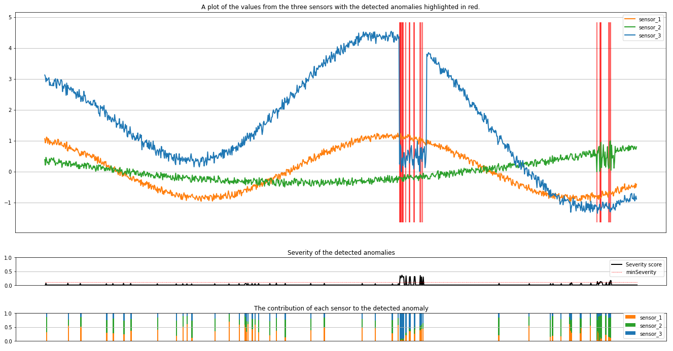
The plots show the raw data from the sensors (inside the inference window) in orange, green, and blue. The red vertical lines in the first figure show the detected anomalies that have a severity greater than or equal to minSeverity.
The second plot shows the severity score of all the detected anomalies, with the minSeverity threshold shown in the dotted red line.
Finally, the last plot shows the contribution of the data from each sensor to the detected anomalies. It helps us diagnose and understand the most likely cause of each anomaly.