Trace, the next AutoDiff

End-to-end Generative Optimization for AI Agents

Getting Started
Trace optimizing a Battleship agent

What is Trace?

Trace is a new AutoDiff-like tool for training AI systems end-to-end with general feedback (like numerical rewards or losses, natural language text, compiler errors, etc.). Trace generalizes the back-propagation algorithm by capturing and propagating an AI system's execution trace. Trace is implemented as a PyTorch-like Python library. Users write Python code directly and can use Trace primitives to optimize certain parts, just like training neural networks!

End-to-End Optimization via LLM

An AI system has many modules. Trace captures the system's underlying execution flow and represents it as a graph (Trace Graph). Trace can then optimize the entire system with general feedback using LLM-based optimizers.

Native Python Support

Trace gives users full flexibility in programming AI systems. Two primitives and wrap over Python objects and functions, making Trace compatible with any Python program and capable of optimizing any mixture of code, string, numbers, and objects, etc.

Platform for Developing New Optimizers

Instead of propagating gradients, Trace propagates Minimal Subgraphs which contains the sufficient information for general computation. This common abstraction allows researchers to develop new optimizers for diverse AI systems.

Consider building an AI agent for the classic Battleship game. In Battleship, a player's goal to hit the ships on a hidden board as fast as possible. To this end, the player must devise strategies to cleverly locate the ships and attack them, instead of slowly enumerating the board. To build an AI agent with Trace, one simply needs to program the workflow of the agent and declare the parameters, just like programming a neural network architecture.
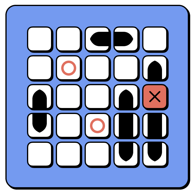
Battleship Game Board

In this example, we will design an agent with two components: a reason function and an act function. To do this, we provide just a basic description of what these two functions should do (reason should analyze the board and act should select a target coordinate). Then we leave the content to be blank and just set those two functions to be trainable (by setting trainable=True). We highlight that, at this point, the agent doesn't know how the Battleship API works. It must not only learn how to play the game, but also learn how to use the unknown API.


    import trace

    @trace.model
    class Agent:

        # this function is not changed by the optimizer
        def __call__(self, map):
            return self.select_coordinate(map).data

        # this function is not changed by the optimizer
        def select_coordinate(self, map):
            plan = self.reason(map)
            output = self.act(map, plan)
            return output

        @trace.bundle(trainable=True)
        def act(self, map, plan):
            """
            Given a map, select a target coordinate in a game.
            X denotes hits, O denotes misses, and . denotes unknown positions.
            """
            return

        @trace.bundle(trainable=True)
        def reason(self, map):
            """
            Given a map, analyze the board in a game.
            X denotes hits, O denotes misses, and . denotes unknown positions.
            """
            return
                                                            

We iteratively train this AI agent to play the game through a simple for loop (see code below). In each iteration, the agent (i.e. policy) sees the board configuration and tries to shoot at a target location. The environment returns in text whether it’s a hit or a miss. Then we run Trace to propagate this environment feedback through agent’s decision logic end-to-end to update the parameters (i.e. the policy is like a two-layer network with a reason layer and an act layer).

These iterations mimic how a human programmer might approach the problem. They run the policy and change the code based on the observed feedback, try different heuristics to solve this problem, and they may rewrite the code a few times to fix any execution errors by using stack traces. The results of the learned policy evaluated on randomly generated held-out games can be found in the top figure of the page. We see the agent very quickly learns a sophisticated strategy to balance exploration and exploitation.


    import trace

    def user_fb_for_placing_shot(board, coords):
        try:
            reward = board.check_shot(coords[0], coords[1])
            new_map = board.get_shots()
            terminal = board.check_terminate()
            return new_map, reward, terminal, f"Got {int(reward)} reward."
        except Exception as e:
            return board.get_shots(), 0, False, str(e)

    board = Battleship()
    obs = trace.node(board.get_shots())  # init observation
    i, max_calls = 0, 10
    while i < max_calls:
        trace.GRAPH.clear()
        try:
            output = policy.select_coordinate(obs)
            obs, reward, terminal, feedback = board.placing_shot(output.data)
        except trace.ExecutionError as e:
            output = e.exception_node
            feedback = output.data
            reward, terminal = 0, False

        if terminal:
            break

        # Update
        optimizer.zero_feedback()
        optimizer.backward(output, feedback)
        optimizer.step(verbose=True)
                                                            

A workflow can have many components and Trace is built to flexibly support Python programs written by a user. Trace creates a unified representation of all the components through a user-defined computational graph, called the Trace graph. This directed acyclic graph is created by using two Trace primitives (node and bundle) to decorate the workflow, which represent node and operations in the graph. Usages of these objects are automatically traced and added to the Trace graph.

Trace primitive can be used to wrap over Python objects as nodes in the graph. The example below shows how different types of Python objects can be included in the Trace graph. Nodes can be marked as trainable, which allows the optimizer to change the content of the node. More importantly, you can perform any Python operations over a node object, and these operations will be traced to construct the Trace graph.

                                        
    import trace
    w = trace.node(3)
    x = trace.node({"learning_rate": 1e-3})
    y = trace.node("You are a helpful assistant.", trainable=True)
    z = trace.node([2, 5, 3])
    z.append(w)
                                

Similarly, allows us to represent Python functions as an operator in the graph. We can describe what the function is doing, and optionally let the optimizer to change the content of this function by setting the trainable flag. You don't need to wrap your Python function in a string to be optimized.

                                    
    import math
    import trace

    @trace.bundle()
    def cbrt(x):  # this function is not changed by the optimizer
        """ Return the cube root of x. """
        return math.cbrt(x)

    @trace.bundle(trainable=True)
    def retrieve_doc(x):  # this function will be optimized
        metric = 'cos_sim'
        return http.api_call(x, metric)
                                

The perspective of primitives makes the graph construction completely automatic, which offers immense flexibility to users. Consider a typical prompt-based LLM task. A program needs to first query the LLM to get a response, and then some post-processing method must be written to extract and verify the LLM response.

The design space of this task is how to construct the best query (prompt) and how to extract the answer from the response. However, these two tasks are tightly coupled. The complexity of the extraction code determines how simple the prompt can be designed and vice versa. Moreover, LLM behaviors are stochastic. When subtle shifts happen in LLM's response, new post-processing code must be written to account for the change.

We can use Trace primitives to wrap two components of this program: both the prompt_template and the extract_answer code. When Predict is constructed and used, a Trace graph is automatically created. The code to this example is in the Big-Bench Hard tab under Showcases.

Trace constructs a computational graph of the user-defined workflow. The graph is an abstraction of the workflow's execution, which might not be the same as the original program. The original program can have complicated logic, but the user can decide what necessary information the computational graph should contain for an optimizer to update the workflow. For an example program:

                                        
    import trace

    x = trace.node(-1.0, trainable=True)
    a = bar(x) # code with complex logic abstracted as an operator by bundle
    b = traced_function()  # traceable codes
    y = a + b
    z = a * y
    z.backward(feedback="Output should be larger.", visualize=True)
                                    

If we visualize during the backward pass, Trace returns to the optimizer a partial graph (Minimal Subgraph) of how the program is run. In this program, we abstracted away all the operations on x inside function bar. However, we can still see how b is generated in traced_function().

Trace allows user to design which part of the workflow they want to present to the LLM optimizer. Users can choose to present as much information (i.e., a complete picture of the workflow) or as little information (i.e., only the most crucial part of the workflow) as possible.
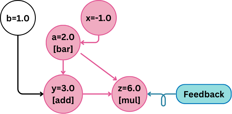
Trace graph

An optimizer works with this Trace graph presented by Trace (which is called the trace feedback in the paper), which gives structural information of computation process. In the paper, we present an initial design of an optimizer (OptoPrime) that represents the Trace graph as a code debugging report, and ask an LLM to change part of the graph that is marked as trainable=True according to feedback.

                                        
    #Code:
    a = bar(x)
    y = add(b, a)
    z = mul(a, y)

    #Definitions:
    [mul] This is a multiply operator
    [add] This is an add operator.
    [bar] This is a method that does negative scaling.

    #Inputs:
    b=1.0

    #Others:
    a=2.0
    y=3.0

    #Output
    z=6.0

    #Variable
    x=-1.0

    #Feedback:
    Output should be larger.
                                    

This debug report is presented an LLM and the LLM is asked to propose changes to the variables. Note that this report may look like the actual program, but is not the same as the python program. Even though any user can directly present the FULL python program to an LLM and ask it to change, it would be (1) Difficult to control LLM to only change the relevant/necessary part; (2) Hard to flexibly specify which part of the workflow LLMs should focus on.

The design of Trace is based on a new mathematical setup of iterative optimization, which we call Optimization with Trace Oracle (OPTO). In OPTO, an optimizer selects parameters and receives a computational graph of execution trace as well as feedback on the computed output. This formulation is quite general and can describe many end-to-end optimization problems in AI systems, beyond neural networks. This key finding gives Trace the foundation to effectively optimize AI systems.

Definition of OPTO : An OPTO problem instance is defined by a tuple $(\Theta, \omega, T)$, where $\Theta$ is the parameter space, $\omega$ is the context of the problem, and $T$ is a Trace Oracle. In each iteration, the optimizer selects a parameter $\theta\in\Theta$, which can be heterogeneous. Then the Trace Oracle $T$ returns a trace feedback, denoted as $\tau = (f,g)$, where $g$ is the execution trace represented as a DAG (the parameter is contained in the root nodes of $g$), and $f$ is the feedback provided to exactly one of the output nodes of $g$. Finally, the optimizer uses the trace feedback $\tau$ to update the parameter according to the context $\omega$ and proceeds to the next iteration.


Here is how some existing problems can be framed as OPTO problems.

  • Neural network with back-propagation: The parameters are the weights. $g$ is the neural computational graph and $f$ is the loss. An example context $\omega$ can be "Minimize loss". The back-propagation algorithm can be embedded in the OPTO optimizer, e.g., an OPTO optimizer can use $\tau$ to compute the propagated gradient at each parameter, and apply a gradient descent update.
  • RL: The parameters are the policy. $g$ is the trajectory (of states, actions, rewards) resulting from running the policy in a Markov decision process; that is, $g$ documents the graphical model of how an action generated by the policy, applied to the transition dynamics which then returns the observation and reward, etc. $f$ can be the termination signal or a success flag. $\omega$ can be "Maximize return" or "Maximize success".
  • Prompt Optimization of an LLM Agent: The parameters are the prompt of an LLM workflow. $g$ is the computational graph of the agent and $f$ is the feedback about the agent's behavior (which can be scores or natural language). $\omega$ can be "Maximize score" or "Follow the feedback".

We design Trace as a tool to efficiently convert the optimization of AI systems into OPTO problems. Trace acts as the Trace Oracle in OPTO, which is defined by the usage of Trace primitives in the user's program. Trace implements the trace feedback returned by the Trace Oracle as the Trace Graph, which defines a general API for AI system optimization. This formulation allows users to develop new optimization algorithms that can be applied to diverse AI systems.

Showcases

We extend the same idea of end-to-end optimization seen in the Battleship example to train more complicated AI systems. Empirical studies showcase Trace's ability to use a single LLM-based optimizer (OptoPrime) to solve diverse problems, from numerical optimization, LLM agents, to robot control, often outperforming specialized optimizers. In these experiments, each iteration makes just one call to an LLM (GPT-4) to optimize graphs of tens of nodes.

For a classical numerical optimization problem, where the objective is to minimize a blackbox function h(x) by choosing a number x, we can directly compare LLM's ability to find the optimal solution against classical numerical optimizers like gradient descent. In this case, the Trace graph is equivalent to the computation graph constructed by PyTorch -- representing the underlying numerical operations over x.

Numerical optimization results

We run 30 trials over different randomly generated problems. All methods see the same randomness. On average, Trace is able to match the best-in-class Adam; on the other hand, without access to the full computational graph, the optimizer alone struggles to find the optimal x.

                                            
    import trace

    program = NumericalProgramSampler(chain_length=7, param_num=1, max_gen_var=4)
    x = trace.node(-1.0, "input_x", trainable=True)

    for i in tqdm(range(n_steps)):
        trace.GRAPH.clear()

        if feedback.lower() == "Success.".lower():
            break

        try:
            output = program(x, seed=program_id)
            feedback = program.feedback(output.data)
        except trace.ExecutionError as e:
            output = e.exception_node
            feedback = output.data

        optimizer.zero_feedback()
        optimizer.backward(output, feedback)
        optimizer.step()
                                            

We tested Trace in a traffic control problem which is an instance of hyper-parameter tuning. We used UXSim to simulate traffic at a four-way intersection, where the trainable parameters are 2 integers in [15,90], which are the green light duration for each direction of traffic flow.

https://raw.githubusercontent.com/toruseo/UXsim/images/gridnetwork_macro.gif

Image sourced from UXSim Website

The feedback is the estimated delay experienced by all vehicles due to intersections, and the goal of an optimizer is to minimize the delay using the fewest number of traffic simulations. To this end, this optimizer must find the right trade-off for temporally distributed and variable demands.

We report the performance of a SOTA heuristic from the traffic control literature, SCATS as well as two black-box optimization techniques: Gaussian Process Minimization (GP) and Particle Swarm Optimization (PSO). All methods use the same starting parameters.

GP and PSO appear bad because 50 iterations are insufficient for their convergence; given enough iterations, both will eventually perform well. Trace is quickly competitive with the SCATS heuristic, whereas OPRO is not. We show the code sketch below. Trace sends a node object into the simulator and let the environment operate on it. The underlying operation logic is automatically revealed to the Trace optimizer.

                                                    
    import trace

    def traffic_simulation(EW_green_time, NS_green_time):
        W = None
        try:
            W = create_world(EW_green_time, NS_green_time)
        except Exception as e:
            e_node = ExceptionNode(
                e,
                inputs={"EW_green_time": EW_green_time, "NS_green_time": NS_green_time},
                description="[exception] Simulation raises an exception with these inputs.",
                name="exception_step",
            )
            return e_node
        W.data.exec_simulation()
        return_dict = analyze_world(W, verbosity)

        return return_dict

    EW_x = trace.node(MIN_GREEN_TIME, trainable=True, constraint=f"[{MIN_GREEN_TIME},{MAX_GREEN_TIME}]")
    NS_x = trace.node(MIN_GREEN_TIME, trainable=True, constraint=f"[{MIN_GREEN_TIME},{MAX_GREEN_TIME}]")

    optimizer.objective = (
                "You should suggest values for the variables so that the OVERALL SCORE is as small as possible.\n"
                + "There is a trade-off in setting the green light durations.\n"
                + "If the green light duration for a given direction is set too low, then vehicles will queue up over time and experience delays, thereby lowering the score for the intersection.\n"
                + "If the green light duration for a given direction is set too high, vehicles in the other direction will queue up and experience delays, thereby lowering the score for the intersection.\n"
                + "The goal is to find a balance for each direction (East-West and North-South) that minimizes the overall score of the intersection.\n"
                + optimizer.default_objective
        )

    for i in range(num_iter):
        result = traffic_simulation(EW_x, NS_x)
        # some steps are skipped for simplicity
        feedback = result.data
        optimizer.zero_feedback()
        optimizer.backward(result, feedback, visualize=True)
        optimizer.step()
                                            

LLM agents today have many components. Most libraries provide optimization tools to optimize a small portion of their workflows, predominantly the prompt that goes into an LLM call. However, for building self-adapting agents that can modify their own behavior, only allowing the change to one part of a workflow but not others seems limiting.

In this experiment, we test Trace's ability in joint prompt optimization and code generation. Specifically, we optimize a given DSPy-based LLM agent and tunes its three components: the meta-prompt prompt_template, a function create_prompt that modifies the prompt with the current question, and a function extract_answer that post-processes the output of an LLM call. We use Big-Bench Hard (BBH) as the problem source. The typical setup of BBH evaluation is 3-shot. We instead choose the more challenging 0-shot setting. The 0-shot setup requires the agent to conform to the correct answer format without any example, challenging for any method that just directly prompts LLM, but not for an agent where a complete workflow is optimized.


We compare Trace with DSPy’s COPRO module (which optimizes the meta-prompt). In the Table below, we show that Trace is able to optimize a DSPy program beyond what DSPy’s COPRO optimizer can offer, especially on algorithmic tasks.

                                                
    import trace

    @trace.model
    class Predict(LLMCallable):
        def __init__(self):
            super().__init__()

            self.demos = []
            self.prompt_template = dedent("""
            Given the fields `question`, produce the fields `answer`.
            ---
            Follow the following format.

            Question:
            Answer:
            ---
            Question: {}
            Answer:""")
            self.prompt_template = trace.node(self.prompt_template, trainable=True)

        @trace.bundle(trainable=True)
        def extract_answer(self, prompt_template, question, response):
            """
            Need to read in the response, which can contain additional thought, delibration and an answer.
            Use code to process the response and find where the answer is.
            Can use self.call_llm("Return the answer from this text: " + response) again to refine the answer if necessary.

            Args:
                prompt_template: The prompt that was used to query LLM to get the response
                question: Question has a text describing the question but also "Options"
                response: LLM returned a string response
            """
            answer = response.split("Answer:")[1].strip()
            return answer

        @trace.bundle(trainable=True)
        def create_prompt(self, prompt_template, question):
            """
            The function takes in a question and then add to the prompt for LLM to answer.
            Args:
                prompt_template: some guidance/hints/suggestions for LLM
                question: the question for the LLM to answer
            """
            return prompt_template.format(question)

        def forward(self, question):
            """
            question: text

            We read in a question and produces a response
            """
            user_prompt = self.create_prompt(self.prompt_template, question)
            response = self.call_llm(user_prompt)
            answer = self.extract_answer(self.prompt_template, question, response)
            return answer


In this example, we want to learn a policy code for controlling a robotic manipulator. Compared with the previous Battleship example, the problem here has a longer horizon, since the policy would need to drive the robot for multiple time steps. Traditionally such a problem is framed as a reinforcement learning (RL) problem and usually learning a policy with RL requires tens of thousands of practice episodes. We show Trace can be used to effectively solve such a problem in just a dozen of episodes -- a 1000X speed up -- since it can end-to-end optimize the control system as opposed to treating the system like a black-box as RL does. We trace the steps of the entire practice episode and perform end-to-end update (using the same optimizer OPTO-Prime) through these steps. In this way, effectively, Trace performs back-propagation through time (BPTT).

We conduct experiments using a simulated Sawyer robot arm in the Meta-World environment of LLF-Bench. The agent policy needs to decide a target pose (end-effector position and the gripper state) for the robot, which will then be used as a set point for a low-level P controller, to perform a pick-and-place task. Each episode has 10 timesteps and tracing through the AI system’s rollout would result in a graph of depth around 30 for an episode. The agent receives intermediate language feedback as observations (from LLF-Bench) and finally feedback about success and return at the end of the episode in texts. Like the Battleship example, we initiate the policy code to be a dummy function and let it adapt through interactions.

We repetitively train the agent start from one initial condition and then test it on 10 new held-out initial conditions for generalization. Trace rapidly learns a robot controller in the MetaWorld simulated environment, that generalizes to new initial conditions. The video shows Trace learns a policy to successfully perform the pick-place task after 13 episodes.

Iteration 0 (Initial Policy)

Iteration 1 (Learned to reach goal but forgot to pick up the object)

Iteration 6 (Dropped the object too early but attempted to recover)

Iteration 13 (100% success rate on configurations unseen in training)

                                                
    import trace

    @trace.bundle(trainable=True)
    def controller(obs):
        """
        A feedback controller that computes the action based on the observation.

        Args:
            obs: (dict) The observation from the environment. Each key is a string (indicating a type of observation) and the value is a list of floats.
        Output:
            action: (list or nd.array) A 4-dimensional vector.
        """
        return [0, 0, 0, 0]

    def rollout(env, horizon, controller):
        """Rollout a controller in an env for horizon steps."""
        traj = dict(observation=[], action=[], reward=[], termination=[], truncation=[], success=[], input=[], info=[])

        # Initialize the environment
        obs, info = env.reset()
        traj["observation"].append(obs)

        # Rollout
        for t in range(horizon):
            controller_input = obs["observation"]
            error = None
            try:  # traced
                action = controller(controller_input)
                next_obs, reward, termination, truncation, info = env.step(action)
            except trace.ExecutionError as e:
                error = e
                break

            if error is None:
                # code skipped...logging
                if termination or truncation or info["success"]:
                    break
                obs = next_obs
        return traj, error

    optimizer = optimizer_cls(controller.parameters())
    env = TracedEnv(env_name, seed=seed, feedback_type=feedback_type, relative=relative)

    print("Optimization Starts")
    for i in range(n_optimization_steps):
        # Rollout and collect feedback
        traj, error = rollout(env, horizon, controller)
        feedback = construct_feedback(traj, error)

        # we provide a task-specific single-line hint for the optimizer
        optimizer.objective = hint + optimizer.default_objective

        # Optimization step
        optimizer.zero_feedback()
        optimizer.backward(target, feedback)
        optimizer.step()


Team

Trace includes contributions from the following people listed alphabetically. We are also thankful to the many people behind the scenes who provided support and feedback in the form of suggestions, Github issues, and reviews.

Ching-An Cheng

Senior Researcher
Microsoft Research

Allen Nie

PhD
Stanford University

Adith Swaminathan

Principal Researcher
Microsoft Research