Geospatial Data

When working with geospatial data, it is generally desirable to include a map in the background to provide geographic context. One way to do this is to use a map image as a background texture. Data can be rendered as a planar or spherical projection.

Planar Projection

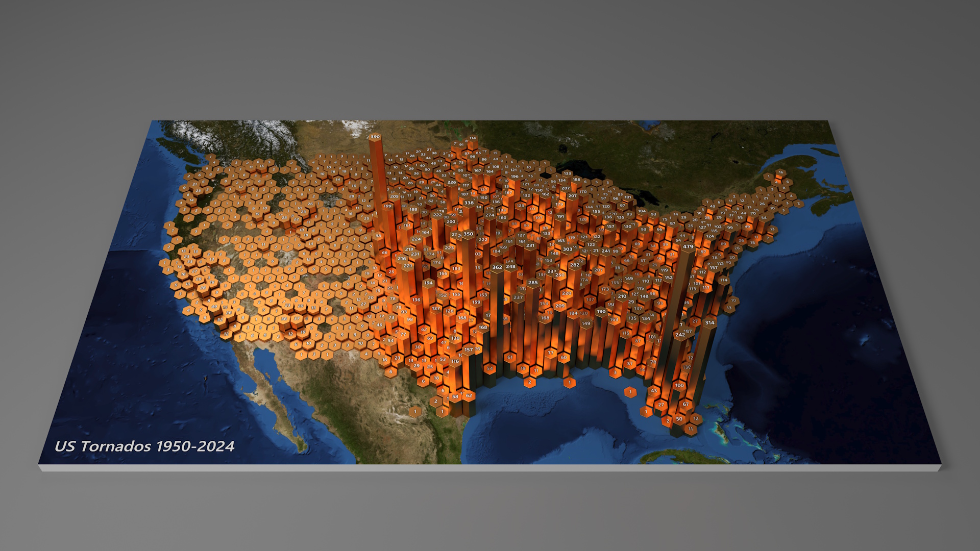
This example shows tornado occurrences across the United States from 1950 to 2024, rendered as hexagonal bins on top of a Mercator-projected map image. The hex bins are sized by count of tornadoes in each cell.

Imagery courtesy of the U.S. Geological Survey National Map. Tornado data courtesy of the NOAA Storm Prediction Center.

View in Online Editor

Projection

A Mercator projection is defined to convert longitude and latitude in degrees to projected x and y coordinates in the [-1, 1] range:

"projections": [
  {
    "name": "projection",
    "type": "mercator"
  }
]

The projection supports optional center, scale and translate properties. In this example, the projection is left at its default center of [0,0] and scale of 1. The projected coordinates are instead subsequently adjusted using formula transforms to center the map and fill the viewport.

Background Image

A map image in a Mercator projection is loaded and its corner coordinates (longitude/latitude) are projected to Mercator coordinates using the geopoint transform and the projection. A pair of extent transforms captures these projected extents, which are used in two subsequent formula transforms to center the coordinates at the midpoint of each axis. A second pair of extent transforms captures these centered extents so they can be used to define a scale.

"images": [
  {"name": "map", "url": "img/..."}
],

"data": [
  {
    "name": "image",
    "values": [
      { "lon": -129.375, "lat": 21.943046 },
      { "lon": -61.875, "lat": 52.48278 }
    ],
    "transform": [
      {"type": "geopoint", "projection": "projection", "fields": ["lon", "lat"], "as": ["xc", "zc"]},
      {"type": "extent", "field": "xc", "signal": "imageExtentX"},
      {"type": "extent", "field": "zc", "signal": "imageExtentZ"},
      {"type": "formula", "expr": "datum.xc-(imageExtentX[0]+imageExtentX[1])/2", "as": "xc"},
      {"type": "formula", "expr": "datum.zc-(imageExtentZ[0]+imageExtentZ[1])/2", "as": "zc"}, 
      {"type": "extent", "field": "xc", "signal": "imageCenteredX"},
      {"type": "extent", "field": "zc", "signal": "imageCenteredZ"}
    ]
  }
]

Data

The data is loaded from a CSV file. Each row contains a longitude and latitude, which are projected using a geopoint transform. A pair of formula transforms centers the projected coordinates by subtracting the mid-point of the image extent. The image plane is defined as the xz plane (x corresponds to longitude, z corresponds to latitude). The z coordinate is flipped for right-hand coordinates, such that an increase in latitude corresponds to a decrease in the z coordinate. The hexbin transform divides the image extent into a hex grid and assigns each data row to a hex cell, outputting the cell bounds as x0, x1, z0, and z1. By using the image extent, we ensure the hex bins are sized consistently, regardless of the data extent.

{
  "name": "table",
  "url": "data/ustornados_1950-2024.csv",
  "transform": [
    {"type": "geopoint", "projection": "projection", "fields": ["slon", "slat"], "as": ["xc", "zc"] },
    {"type": "formula", "expr": "datum.xc-(imageExtentX[0]+imageExtentX[1])/2", "as": "xc"},
    {"type": "formula", "expr": "(imageExtentZ[0]+imageExtentZ[1])/2-datum.zc", "as": "zc"},
    {
      "type": "hexbin",
      "fields": ["xc", "zc"],
      "extent": {"signal": "[[imageCenteredX[0],imageCenteredZ[0]],[imageCenteredX[1],imageCenteredZ[1]]]"},
      "maxbins": {"signal": "maxbins"},
      "as": ["x0", "x1", "z0", "z1"]
    }
  ]
}

Aggregation

The hex-binned data is aggregated to count the number of rows in each hex cell:

{
  "name": "aggregate",
  "source": "table",
  "transform": [
    {
      "type": "aggregate",
      "groupby": ["x0", "x1", "z0", "z1"],
      "ops": ["count"],
      "as": ["count"]
    }
  ]
}

Scales

A single linear scale maps the larger of the two projected, centered image extents to fill the plot dimensions (width), ensuring uniform scaling across both x and z axes. If a default camera is used, the plot will be sized to fit the image, so the longest dimension will fill the vertical viewport. Since the data has been centered using the image extent mid-point, the scale domain is symmetric around zero. A second scale maps the count to the y axis (height):

"scales": [
  {
    "name": "xzscale",
    "type": "linear",
    "domain": {"signal": "imageCenteredX[1]>imageCenteredZ[1]?imageCenteredX:imageCenteredZ"},
    "range": "width"
  },
  {
    "name": "yscale",
    "type": "linear",
    "domain": {"data": "aggregate", "field": "count"},
    "range": "height"
  }
]

Marks

The map image is rendered as a textured rectangle in the xz plane, positioned using the image extents through the xzscale. The z texture coordinate is flipped for right-hand coordinates:

{
  "type": "rect",
  "geometry": "xzrect",
  "encode": {
    "enter": {
      "x":  {"scale": "xzscale", "signal": "imageCenteredX[0]"},
      "x2": {"scale": "xzscale", "signal": "imageCenteredX[1]"},
      "z":  {"scale": "xzscale", "signal": "imageCenteredZ[0]"},
      "z2": {"scale": "xzscale", "signal": "imageCenteredZ[1]"},
      "fill": {"image": "map", "texScale": {"z": {"value": -1}}}
    }
  }
}

The aggregated count for each hex cell is rendered as a single hexagonal prism, positioned using the hex cell bounds and scaled vertically by count. A rounding radius is set at 2% of the hex cell size:

{
  "type": "rect",
  "geometry": "hexprismsdf",
  "material": "metal",
  "from": {"data": "aggregate"},
  "encode": {
    "enter": {
      "x": {"scale": "xzscale", "field": "x0", "offset": {"signal": "0.04*width/maxbins"}},
      "x2": {"scale": "xzscale", "field": "x1", "offset": {"signal": "-0.04*width/maxbins"}},
      "y": {"value": 10},
      "y2": {"scale": "yscale", "field": "count", "offset": 10},
      "z": {"scale": "xzscale", "field": "z0", "offset": {"signal": "0.04*width/maxbins"}},
      "z2": {"scale": "xzscale", "field": "z1", "offset": {"signal": "-0.04*width/maxbins"}},
      "rounding": {"signal": "0.02*width/maxbins"},
    }
  }
}

Text labels showing the count are positioned on top of each hex prism, rotated to face upward:

{
  "type": "text",
  "from": {"data": "aggregate"},
  "encode": {
    "enter": {
      "x": {"scale": "xzscale", "signal": "(datum.x0+datum.x1)/2"},
      "y": {"scale": "yscale", "field": "count", "offset": 10.01},
      "z": {"scale": "xzscale", "signal": "(datum.z0+datum.z1)/2"},
      "text": {"field": "count"},
      "angleX": {"value": 90}
    }
  }
}

Spherical Projection

This example shows worldwide earthquakes from 2000 to 2025. The epicenters are positioned above a globe, with the altitude representing an exaggerated depth. The size and color represent magnitude. The globe is textured with a land/ocean mask image to provide geographic context.

Blue Marble imagery courtesy of NASA Earth Observatory. Earthquake data courtesy of U.S. Geological Survey, Earthquake Hazards Program.

View in Online Editor

Data

The earthquake data contains longitude, latitude, depth (km), and magnitude for each event. The depth is normalized to the Earth's average radius, scaled by altitudeScaling, and added to the unit sphere radius to position the epicentre above the globe surface. The geopoint3d transform converts longitude, latitude, and altitude to spherical coordinates. Size is calculated by scaling magnitude exponentially, such that each magnitude step doubles the size. The minimum magnitude in the dataset is 5.

"transform": [
  {"type": "formula", "expr": "1+altitudeScaling*datum.depth/6371", "as": "altitude"},
  {"type": "geopoint3d", "fields": ["longitude", "latitude", "altitude"], "as": ["x", "y", "z"]},
  {"type": "formula", "expr": "pow(2,datum.mag-5)", "as": "r"}
]

Marks

The globe is rendered as a sphere with a land/ocean mask as the fill texture:

{
  "type": "rect",
  "geometry": "sphere",
  "material": "metal",
  "encode": {
    "enter": {
      "xc": {"signal": "width/2"},
      "zc": {"signal": "depth/2"},
      "yc": {"signal": "height/2"},
      "width": {"signal": "globeRadius*2"},
      "fuzz": {"value": 1},
      "fill": {"image": "map"}
    }
  }
}

Each earthquake is rendered as a sphere positioned using x, y and z, sized by r, scaled by globeRadius, and offset by the globe position:

{
  "type": "rect",
  "geometry": "sphere",
  "from": {"data": "table"},
  "encode": {
    "enter": {
      "xc": {"field": "x", "mult": {"signal": "globeRadius"}, "offset": {"signal": "width/2"}},
      "zc": {"field": "z", "mult": {"signal": "globeRadius"}, "offset": {"signal": "depth/2"}},
      "yc": {"field": "y", "mult": {"signal": "globeRadius"}, "offset": {"signal": "height/2"}},
      "width": {"signal": "datum.r"},
      "fill": {"scale": "fill", "field": "mag"}
    }
  }
}