Training an audio keyword spotter with PyTorch

by Chris Lovett

This tutorial will show you how to train a keyword spotter using PyTorch. A keyword spotter listens to an audio stream from a microphone and recognizes certain spoken keywords. Since it is always listening there is good reason to find a keyword spotter that can run on a very small low-power co-processor so the main computer can sleep until a word is recognized. The ELL compiler makes that possible. In this tutorial you will train a keyword spotter using the the speech commands dataset which contains 65,000 recordings of 30 different keywords (bed, bird, cat, dog, down, eight, five, four, go, happy, house, left, marvin, nine, no, off, on, one, right, seven, sheila, six, stop, three, tree, two, up, wow, yes, zero) each about one second long.

This is the dataset used to train the models in the speech commands model gallery. The Getting started with keyword spotting on the Raspberry Pi tutorial uses these models. Once you learn how to train a model you can then train your own custom model that responds to different keywords, or even random sounds, or perhaps you want just a subset of the 30 keywords for your application. This tutorial shows you how to do that.

Before you begin

Complete the following steps before starting the tutorial.

Install ELL on your computer (Windows, Ubuntu Linux, macOS).

What you will need

Laptop or desktop computer with at least 16 GB of RAM.
Optional NVidia Graphics Card that supports CUDA. You will get great results with a GTX 1080 which is commonly used for training neural networks.
The NVidia CUDA 10.0 SDK from https://developer.nvidia.com/cuda-downloads.

Overview

The picture below illustrates the process you will follow in this tutorial. First you will convert the wav files into a big training dataset using a featurizer. This dataset is the input to the training process which outputs a trained keyword spotter. The keyword spotter can then be verified by testing.

process

Training a Neural Network is a computationally intensive task that takes millions or even billions of floating point operations. That is why you probably want to use CUDA accelerated training. Fortunately, audio models train pretty quickly. On an NVidia 1080 graphic card the 30 keyword speech_commands dataset trains in about 3 minutes using PyTorch. Without CUDA the same training takes over 2.5 hours on an Intel Core i7 CPU.

ELL Root

After you have installed and built the ELL compiler, you also need to set an environment variable named ELL_ROOT that points to the location of your ELL git repo, for example:

[Linux] export ELL_ROOT="~/git/ell"

[Windows] set ELL_ROOT=d:\git\ell

Subsequent scripts depend on this path being set correctly. Now make a new working folder:

mkdir tutorial
cd tutorial

Installing PyTorch

Installing PyTorch with CUDA is easy to do using your Conda environment. If you don’t have a Conda environment, see the ELL setup instructions (Windows, Ubuntu Linux, macOS).

You may want to create a new Conda environment for PyTorch training, or you can add PyTorch to your existing one. You can create a new environment easily with this command:

conda create -n torch python=3.6

Activate it

[Linux] source activate torch
[Windows] activate torch

Then follow the PyTorch setup instructions for Anaconda and your version of CUDA as described on this page: https://pytorch.org/get-started/locally/.

Installing pyaudio

This tutorial uses pyaudio which can be installed using:

[Linux] sudo apt-get install python-pyaudio python3-pyaudio portaudio19-dev && pip install pyaudio
[Windows] pip install pyaudio
[macOS] brew install portaudio && pip install pyaudio

Helper Python Code

This tutorial uses python scripts located in your ELL git repo under tools/utilities/pythonlibs/audio and tools/utilities/pythonlibs/audio/training. When you see a python script referenced below like make_training_list.py, just prefix that with the full path to that script your ELL git repo.

Downloading the Training Data

Next, you will need to download the training data set:

Speech Commands Dataset (1.4 gigabytes)

Google crowd sourced the creation of these recordings so you get a nice variety of voices. Google released it under the Creative Commons BY 4.0 license.

Go ahead and download that file and move it into a folder named audio then unpack it using this Linux command:

tar xvf speech_commands_v0.01.tar.gz

On Windows you can use the Windows Subsystem for Linux to do the same. Alternatively, you can install 7-zip. 7-zip will install a new menu item so you can right click the speech_commands_v0.01.tar.gz and select “Extract here”. The total disk space required for the uncompressed files is about 2 GB. When complete your audio folder should contain 30 folders plus one named background_noise. You should also see the following additional files:

validation_list.txt - the list of files that make up the validation set
testing_list.txt - the list of files in the testing set

Lastly, you will need to create the training_list.txt file containing all the wav files (minus the validation and test sets) which you can do with this command:

python make_training_list.py --wav_files audio --max_files_per_directory 1600
copy audio\categories.txt .

Where audio is the path to your unpacked speech command wav files. This will also create a categories.txt file in the same folder. This file lists the names of the keywords (directories) found in the audio folder. Copy that file to your working tutorial folder.

Note that the command line above includes the option --max_files_per_directory 1600. This options limits the training list to a maximum of 1600 files per subdirectory and will result in a training dataset of around 1.2 GB (using the make_dataset command line options shown below). Feel free to try other numbers here or remove the limit entirely to use every available file for training. You will notice there are not exactly the same number of training files in each subdirectory, but that is ok. Without any limits the full speech_commands training dataset file will be about 1.6 GB and the make_training_list.py script may use up to 6 gb RAM to get the job done.

As you can see you can try different sized training datasets. When you are ready to experiment, figure out which gives the best results, all the training files, or a subset.

Create a Featurizer Model

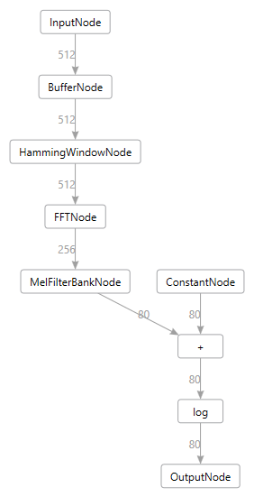
As shown in the earlier tutorial the featurizer model is a mel-frequency cepstrum (mfcc) audio transformer which preprocesses audio input, preparing it for use by the training process.

This featurizer is created as an ELL model using the make_featurizer command:

python make_featurizer.py --sample_rate 16000 --window_size 512 --input_buffer_size 512 --hamming_window --filterbank_type mel --filterbank_size 80 --filterbank_nfft 512 --nfft 512 --log --auto_scale

The reason for the --sample_rate 16000 argument is that small low powered target devices might not be able to record and process audio at very high rates.

So while your host PC can probably do 96kHz audio and higher just fine, this tutorial shows you how to down sample the audio to something that will run on a tiny target device. The main point being that you will get the best results if you train the model on audio that is sampled at the same rate that your target device will be recording.

The --auto_scale option converts raw integer audio values to floating point numbers in the range [-1, 1].

You should see a message saying “Saving featurizer.ell” and if you print this using the following command line:

[Linux] $ELL_ROOT/build/bin/print -imap featurizer.ell
[Windows] %ELL_ROOT%\build\bin\release\print -imap featurizer.ell -fmt dgml -of graph.dgml

then you will see the following nodes:

featurizer

You can now compile this model using the ELL model compiler to run on your PC using the familiar wrap command:

[Windows] python %ELL_ROOT%\tools\wrap\wrap.py --model_file featurizer.ell --outdir compiled_featurizer --module_name mfcc

[Linux] python $ELL_ROOT/tools/wrap/wrap.py --model_file featurizer.ell --outdir compiled_featurizer --module_name mfcc

Then you can build the compiled_featurizer folder using cmake as done in prior tutorials. You will do this a lot so it might be handy to create a little batch or shell script called makeit that contains the following:

Windows:

mkdir build
cd build
cmake -G "Visual Studio 16 2019" -A x64 ..
cmake --build . --config Release
cd ..

Linux:

#!/bin/bash
mkdir build
cd build
cmake ..
make
cd ..

So compiling a wrapped ELL model is now this simple:

pushd compiled_featurizer
makeit
popd

Create the Dataset using the Featurizer

Now you have a compiled featurizer, so you can preprocess all the audio files using this featurizer and create a compressed numpy dataset with the result. This large dataset will contain one row per audio file, where each row contains all the featurizer output for that file. The featurizer output is smaller than the raw audio, but it will still end up being a pretty big file, (about 1.2 GB). Of course it depends how many files you include in the set. Remember for best training results the more files the better, so you will use the training_list.txt you created earlier which selected 1600 files per keyword. You need three datasets created from each of the list files in your audio folder using make_dataset as follows:

python make_dataset.py --list_file audio/training_list.txt --featurizer compiled_featurizer/mfcc --window_size 40 --shift 40
python make_dataset.py --list_file audio/validation_list.txt --featurizer compiled_featurizer/mfcc --window_size 40 --shift 40
python make_dataset.py --list_file audio/testing_list.txt --featurizer compiled_featurizer/mfcc --window_size 40 --shift 40

Where the audio folder contains your unpacked .wav files. If your audio files are in a different location then simply provide the full path to it in the above commands.

Creating the datasets will take a while, about 10 minutes or more, so now is a great time to grab a cup of tea. It will produce three files in your working folder named training.npz, validation.npz and testing.npz which you will use below.

Note that make_training_list.py skipped the _background_noise folder. But make_dataset.py has options to use that background noise to randomly mix in with each training word. By default make_dataset.py does not do that. But you can experiment with this and see if it helps or not.

Train the Keyword Spotter

You can now finally train the keyword spotter using the train_classifier script:

python train_classifier.py --architecture GRU --num_layers 2 --dataset . --use_gpu --outdir .

This script will use PyTorch to train a GRU based model using the datasets you created earlier then it will export an onnx model from that. The file will be named KeywordSpotter.onnx and if all goes well you should see console output like this:

Loading .\testing_list.npz...
Loaded dataset testing_list.npz and found sample rate 16000, audio_size 512, input_size 80, window_size 40 and shift 40
Loading .\training_list.npz...
Loaded dataset training_list.npz and found sample rate 16000, audio_size 512, input_size 80, window_size 40 and shift 40
Loading .\validation_list.npz...
Loaded dataset validation_list.npz and found sample rate 16000, audio_size 512, input_size 80, window_size 40 and shift                                          40
Training model GRU128KeywordSpotter.pt
Training 2 layer GRU 128 using 46256 rows of featurized training input...
RMSprop (
Parameter Group 0
    alpha: 0
    centered: False
    eps: 1e-08
    lr: 0.001
    momentum: 0
    weight_decay: 1e-05
)
Epoch 0, Loss 1.624, Validation Accuracy 48.340, Learning Rate 0.001
Epoch 1, Loss 0.669, Validation Accuracy 78.581, Learning Rate 0.001
Epoch 2, Loss 0.538, Validation Accuracy 88.623, Learning Rate 0.001
Epoch 3, Loss 0.334, Validation Accuracy 91.423, Learning Rate 0.001
Epoch 4, Loss 0.274, Validation Accuracy 92.041, Learning Rate 0.001
Epoch 5, Loss 0.196, Validation Accuracy 93.945, Learning Rate 0.001
Epoch 6, Loss 0.322, Validation Accuracy 93.652, Learning Rate 0.001
Epoch 7, Loss 0.111, Validation Accuracy 94.548, Learning Rate 0.001
Epoch 8, Loss 0.146, Validation Accuracy 95.296, Learning Rate 0.001
Epoch 9, Loss 0.109, Validation Accuracy 95.052, Learning Rate 0.001
Epoch 10, Loss 0.115, Validation Accuracy 95.492, Learning Rate 0.001
Epoch 11, Loss 0.116, Validation Accuracy 95.931, Learning Rate 0.001
Epoch 12, Loss 0.064, Validation Accuracy 95.866, Learning Rate 0.001
Epoch 13, Loss 0.159, Validation Accuracy 95.736, Learning Rate 0.001
Epoch 14, Loss 0.083, Validation Accuracy 95.898, Learning Rate 0.001
Epoch 15, Loss 0.094, Validation Accuracy 96.484, Learning Rate 0.001
Epoch 16, Loss 0.056, Validation Accuracy 95.801, Learning Rate 0.001
Epoch 17, Loss 0.096, Validation Accuracy 95.964, Learning Rate 0.001
Epoch 18, Loss 0.019, Validation Accuracy 96.305, Learning Rate 0.001
Epoch 19, Loss 0.140, Validation Accuracy 96.501, Learning Rate 0.001
Epoch 20, Loss 0.057, Validation Accuracy 96.094, Learning Rate 0.001
Epoch 21, Loss 0.025, Validation Accuracy 96.289, Learning Rate 0.001
Epoch 22, Loss 0.037, Validation Accuracy 95.947, Learning Rate 0.001
Epoch 23, Loss 0.008, Validation Accuracy 96.191, Learning Rate 0.001
Epoch 24, Loss 0.050, Validation Accuracy 96.419, Learning Rate 0.001
Epoch 25, Loss 0.010, Validation Accuracy 96.257, Learning Rate 0.001
Epoch 26, Loss 0.014, Validation Accuracy 96.712, Learning Rate 0.001
Epoch 27, Loss 0.044, Validation Accuracy 96.159, Learning Rate 0.001
Epoch 28, Loss 0.011, Validation Accuracy 96.289, Learning Rate 0.001
Epoch 29, Loss 0.029, Validation Accuracy 96.143, Learning Rate 0.001
Trained in 299.81 seconds
Training accuracy = 99.307 %
Evaluating GRU keyword spotter using 6573 rows of featurized test audio...
Saving evaluation results in '.\results.txt'
Testing accuracy = 93.673 %
saving onnx file: GRU128KeywordSpotter.onnx

So here you see the model has trained well and is getting an evaluation score of 93.673% using the testing_list.npz dataset. The testing_list contains files that the training_list never saw before so it is expected that the test score will always be lower than the final training accuracy (99.307%). The real trick is increasing that test score. This problem has many data scientists employed around the world!

Importing the ONNX Model

In order to try your new model using ELL, you first need to import it from ONNX into the ELL format as follows:

[Linux] python $ELL_ROOT/tools/importers/onnx/onnx_import.py GRU128KeywordSpotter.onnx
[Windows] python %ELL_ROOT%\tools\importers\onnx\onnx_import.py GRU128KeywordSpotter.onnx

This will generate an ELL model named GRU128KeywordSpotter.ell which you can now compile using similar technique you used on the featurizer:

[Linux] python $ELL_ROOT%/tools/wrap/wrap.py --model_file GRU128KeywordSpotter.ell --outdir KeywordSpotter --module_name model
[Windows] python %ELL_ROOT%\tools\wrap\wrap.py --model_file GRU128KeywordSpotter.ell --outdir KeywordSpotter --module_name model

then compile the resulting KeywordSpotter project using your new makeit command:

pushd KeywordSpotter
makeit
popd

Testing the Model

So you can now take the new compiled keyword spotter for a spin and see how it works. You can measure the accuracy of the ELL model using the testing list. The test_ell_model.py script will do that:

python test_ell_model.py --classifier KeywordSpotter/model --featurizer compiled_featurizer/mfcc --sample_rate 16000 --list_file audio/testing_list.txt --categories categories.txt --reset --auto_scale

This is going back to the raw .wav file input and refeaturizing each .wav file using the compiled featurizer, processing each file in random order. This is similar to what you will do on your target device while processing microphone input. As a result this test pass will take a little longer (about 2 minutes). You will see every file scroll by telling you which one passed or failed with a running pass rate. The last page of output should look something like this:

...
Saving 'results.json'
Test completed in 157.65 seconds
6090 passed, 483 failed, pass rate of 92.65 %
Best prediction time was 0.0 seconds

The final pass rate printed here is 92.65% which is close to the pytorch test accuracy of 93.673%.

But how will this model perform on a continuous stream of audio from a microphone? You can try this out using the following tool:

[Linux] python $ELL_ROOT/tools/utilities/pythonlibs/audio/view_audio.py --classifier KeywordSpotter\model --featurizer compiled_featurizer/mfcc --categories categories.txt --sample_rate 16000 --threshold 0.8 --auto_scale

[Windows] python %ELL_ROOT%\tools\utilities\pythonlibs\audio\view_audio.py --classifier KeywordSpotter\model --featurizer compiled_featurizer/mfcc --categories categories.txt --sample_rate 16000 --threshold 0.8 --auto_scale

Speak some words from categories.txt slowly and clearly. You will find that the accuracy is not as good, it recoginizes the first word you speak, but nothing else. If you run the test_ell_model.py script without “–reset” argument then the test is run as one continuous steam of audio with no model reset between each .wav file. In this case you will see the test score drop to about 70%. So why is this? Well, remember the trainer has one row per wav recording and this helps the trainer know when to reset the GRU node hidden state. See the init_hidden method. But in live audio how do you know when one word stops and another starts? Sometimes spoken words blur together. How does ELL then know when to reset the GRU nodes hidden state? By default ELL does not reset the hidden state so the GRU state blurs together over time and gets confused especially if there is no clear silence between consecutive words.

So how can you fix this? Well, this is where Voice Activity Detection (VAD) can come in handy. ELL actually has a node called VoiceActivityDetectorNode that you can add to the model. The input is the same featurizer input that the classifier uses, and the output is an integer value 0 if there is no activity detected and 1 if there is activity. This output signal can then be piped into the GRU nodes as a “reset_trigger”. The GRU nodes will then reset themselves when they see that trigger change from 1 to 0 (the end of a word). To enable this you will need to edit the ELL GRU128KeywordSpotter.ell file using the add_vad.py script:

python add_vad.py GRU128KeywordSpotter.ell --sample_rate 16000 --window_size 512 --tau_up 1.5 --tau_down 0.09 --large_input 4 --gain_att 0.01 --threshold_up 3.5 --threshold_down 0.9 --level_threshold 0.02

This will edit the ELL model, remove the dummy reset triggers on the two GRU nodes and replace them with a VoiceActivityDetectorNode. Your new GRU128KeywordSpotter.ell should now look like this:

graph

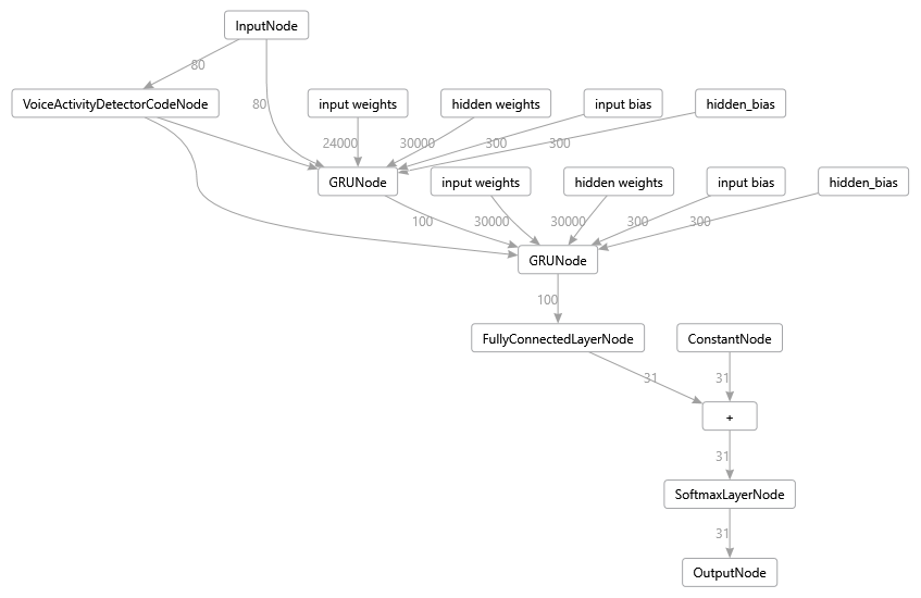
Note: you can use the following tool to generate these graphs:

[Linux] $ELL_ROOT/build/bin/release/print -imap GRU128KeywordSpotter.ell -fmt dot -of graph.dot
[Windows] %ELL_ROOT%\build\bin\release\print -imap GRU128KeywordSpotter.ell -fmt dgml -of graph.dgml

And you can view graph.dgml using Visual Studio. On Linux you can use the dot format which can be viewed using GraphViz.

You can now compile this new GRU128KeywordSpotter.ell model using wrap.py as before and try it out. You should see the test_ell_model accuracy increase back up from 70% to about 85%. The VoiceActivityDetector is not perfect on all the audio test samples, especially those with high background noise. The VoiceActivityDetector has many parameters that you can see in add_vad.py. These parameters can be tuned for your particular device to get the best result. You can use the <ELL_ROOT>/tools/utilities/pythonlibs/audio/vad_test.py tool to help with that.

You can also use the view_audio.py script again and see how it behaves when you speak the 30 different keywords listed in categories.txt. You should notice that it works better now because of the VoiceActivityDetection whereas previously you had to click “stop” and “record” to reset the model. Now it resets automatically and is able to recognize the next keyword after a small silence. You still cannot speak the keywords too quickly, so this solution is not perfect. Understanding full conversation speech is a different kind of problem that requires bigger models and audio datasets that include whole phrases.

VAD Tuning

The add_vad.py script takes many parameters that you may need to tune for your particular microphone. To do this use the following tool:

tools/utilities/pythonlibs/audio/vad_test.py

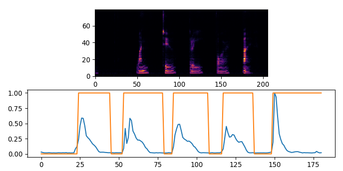
This tool takes the featurizer.ell and generates vad.ell models matching the given parameters you provide in the dialog, and it will test that on a given wav file. So record wav files off the STM32F469-disco of you speaking a few words (in a quiet place) and run them, then calibrate the vad.ell model parameters until the vad output detects words and silence correctly. You are done when the graph looks like this. You may also need to configure the microphone gain on your device. Specifically you should see the Orange VAD signal nicely frame each word spoken.

vad

Use --help on the add_vad.py command line to see what each parameter means.

Experimenting

The train_classifier.py script has a number of other options you can play with including number of epochs, batch_size, learning_rate, and the number of hidden_units to use in the GRU layers. Note that training also has an element of randomness to it, so you will never see the exact same numbers even when you retrain with the exact same parameters. This is due to the Stochastic Gradient Descent algorithm that is used by the trainer.

The neural network you just trained is described by the KeywordSpotter class in the train_classifier.py script. You can see the __init__ method of the GRU128KeywordSpotter class creating two GRU nodes and a Linear layer which are used by the forward method as follows:

    def forward(self, input):
        # input has shape: [seq,batch,feature]
        gru_out, self.hidden1 = self.gru1(input, self.hidden1)
        gru_out, self.hidden2 = self.gru2(gru_out, self.hidden2)
        keyword_space = self.hidden2keyword(gru_out)
        result = F.log_softmax(keyword_space, dim=2)
        # return the mean across the sequence length to produce the
        # best prediction of which word it found in that sequence.
        # we can do that because we know each window_size sequence in
        # the training dataset contains at most one word and a single
        # word is not spread across multiple training rows
        result = result.mean(dim=0)
        return result

You can now experiment with different model architectures. For example, what happens if you add a third GRU layer? To do that you can make the following changes to the KeywordSpotter class:

Add the construction of the 3rd GRU layer in the __init__ method:
```
 self.gru3 = nn.GRU(hidden_dim, num_keywords)
```
Change the Linear layer to take a different number of inputs since the output of gru3 will now be size num_keywords instead of hidden_dim:
```
 self.hidden2keyword = nn.Linear(num_keywords, num_keywords)
```
Add a third hidden state member in the init_hidden method:
```
 self.hidden3 = None
```

Use this new GRU layer in the forward method right after the gru2.

 gru_out, self.hidden3 = self.gru3(gru_out, self.hidden3)

That’s it! Pretty simple. Now re-run train_classifier as before. Your new model should get an evaluation accuracy that is similar, so the 3rd GRU layer didn’t really help much. But accuracy is not the only measure, you might also want to compare the performance of these two models to see which one is faster. It is often a speed versus accuracy trade off with neural networks which is why you see a speed versus accuracy graph on the ELL Model Gallery.

There are many other things you could try. So long as the trainer still shows a decreasing loss across epochs then it should train ok. You know you have a broken model if the loss never decreases.

As you can see, PyTorch makes it pretty easy to experiment. To learn more about PyTorch see their excellent tutorials.

Hyper-parameter Tuning

So far your training has used all the defaults provided by train_classifier, but an important step in training neural networks is tuning all the training parameters. These include learning_rate, batch_size, weight_decay, lr_schedulers and their associated lr_min and lr_peaks, and of course the number of epochs. It is good practice to do a set of training runs that test a range of different values independently testing all these hyper-parameters. You can probably get a full 1% increase in training accuracy by finding the optimal parameters.

Cleaning the Data

The speech commands dataset contains many bad training files, either total silence, or bad noise, clipped words and some completely mislabelled words. Obviously this will impact your training accuracy. So included in this tutorial is a bad_list.txt file. If you copy that to your speech commands folder (next to your testing_list.txt file) then re-run make_training_list.py with the additional argument --bad_list bad_list.txt then it will create a cleaner test, validation and training list.

Re-run the featurization steps with make_dataset.py and retrain your model and you should now see the test accuracy jump to about 94%. So this is a good illustration of the fact that higher quality labelled data can make a big difference in model performance.

Next steps

That’s it, you just trained your first keyword spotter using PyTorch and you compiled and tested it using ELL, congratulations! You can now use your new featurizer and classifier in your embedded application, perhaps on a Raspberry Pi, or even on an Azure IOT Dev Kit, as shown in the DevKitKeywordSpotter example.

There are also lots of things you can experiment with as listed above. You can also build your own training sets, or customize the speech commands set by simply modifying the the training_list.txt file, then recreate the training_list.npz dataset using make_dataset.py, retrain the model and see how it does.

Another dimension you can play with is mixing noise with your clean .wav files. This can give you a much bigger dataset and a model that performs better in noisy locations. Of course, this depends on what kind of noise you care about. Crowds of people? Industrial machinery? Just the hum of computers and HVAC systems in an Office environment? It depends on your application. You can experiment using the noise files included in the speech_commands dataset. There are some more advanced options on the make_dataset.py script to help with mixing noise in with the audio recordings.

The github speech commands gallery contains some other types of models, some based on LSTM nodes, for example. The GRU architecture does well on smaller sized models, but LSTM hits the highest score when it maximizes the hidden state size.

Troubleshooting

For any PyTorch issues, see https://pytorch.org/.

Exception: Please set your ELL_ROOT environment, as you will be using python scripts from there If you see this error then you need to following ELL setup instructions above and clone the ELL repo, build it, and set an environment variable that points to the location of that repo. This tutorial uses scripts in that repo, and those scripts use the binaries that are built there.