Clustering Domínguez Conde et al 2022

Run NCLUSION

To run NCLUSION from your working direcorty, enter the following bash command.

NOTE: set the --julia_env variable to the relative path to your Julia project environment where NCLUSION is installed.

mkdir -p dominguezconde2022_outputs

. tutorial_scripts/run_nclusion.sh --datapath='tutorial_data/dominguezconde2022/5000hvgs_dominguezconde2022_preprocessed.h5ad' --julia_env='PATH/TO/JULIA/ENV' --data_name='dominguezconde2022' --output_dir='dominguezconde2022_outputs/'

All tutorial output files can be found in the specified output directory: dominguezconde2022_outputs/. All NCLUSION output files can be found in: dominguezconde2022_outputs/outputs/EXPERIMENT_nclusion_dominguezconde2022/DATASET_dominguezconde2022_5000HVGs-88057N/YEAR_MONTH_DATE_TIME/

NOTE: '{YEAR-MONTH-DATE-TIME}' labels in the output path/files corresponds to the time stamp of when the results were generated. The time stamp is added automatically by NCLUSION.

In the output directory, you can find the following output files:

1. dominguezconde2022_5000HVGs-88057N_nclusion-{YEAR-MONTH-DATE-TIME}.csv
   • .csv file that contains the NCLUSION clustering assignments, where each row displays relevant metadata and clustering results for each cell.
   • The 'condition' column displays the cell's experimental condition labels (all cells in this study have the same condition label).
   • The 'cell_id' column displays the cell's unique identifier label.
   • The 'cell_type' column displays the cell's manual cell-type annotation published in this study. This column would be empty for unannotated datasets.
   • The 'called_label' column displays the numerical equivalent of the 'cell_type' label, mapped automatically by NCLUSION.
   • The 'inferred_label' column displays the cell's NCLUSION cluster assignment.
2. 5000G-{YEAR-MONTH-DATE-TIME}-pips.csv
   • .csv file that contains the Posterior Inclusion Probabilities (PIPs) of genes across clusters identified by NCLUSION. PIPs are used as a summary of evidence for a gene being associated with driving the identity of any phenotypic cluster. For a particular cluster, a higher PIP indicates that a gene is more significant to the formation of that cluster.
3. _QuickSummary_{YEAR-MONTH-DATE-TIME}.txt
   • .txt file that contains the input parameters that were used to run NCLUSION.
4. output.jld2
   • .jld2 file that contains all model parameters
5. {YEAR-MONTH-DATE-TIME}-Nk.csv
   • .csv file that contains estimated number of cells in each cluster identified by NCLUSION

NOTE: In the following analyses, clusters are named according to the cluster mapping file: tutorial_scripts/cluster_mapping/dominguezconde_mapping.csv which maps the NCLUSION labels to labels in [1:number of clusters], for aesthetic purposes. This mapping retains NCLUSION cluster memberships.

A. Quantitative Evaluation Metrics

To evaluate the NCLUSION clustering results, the following command calculates various evaluation metrics: Jaccard Indexs, Adjusted Rand Index (ARI) (extrinsic), McIntosh Evenness, and Gini-Simpson Index (intrinsic). Extrinsic metric calculations are dependent on experimental annotations of the data, that act as the "true" labels, while intrinsic metrics do not. Therefore, extrinsic metrics are only calculated when "true" labels are provided in the "cell_type" observation layer of the input AnnData object. The metric calculations are automatically saved to .csv files in the specified output directory. Each file is labeled according to the following format: '{name_of_metric}_NCLUSION_tissueimmuneatlas_5000hvgs.csv'

To calculate evaluation metrics, enter the following command into your bash terminal.

NOTE: be sure to replace --input_path variable with the relative path to your NCLUSION clustering results and --project with the path to your Julia environment where NCLUSION is installed.

python tutorial_scripts/utility_scripts/make_intermediates.py --input_path "/PATH/TO/NCLUSION/CLUSTERING/FILE" --title "NCLUSION Zheng et al 2017" --output_path_file "dominguezconde2022_outputs/" --output_path_figure "dominguezconde2022_outputs/" --output_suffix '' --dataset_ordering_mode "tissueimmuneatlas" --col_sum_threshold '0.15'
  
julia --project='PATH/TO/JULIA/ENV' tutorial_scripts/utility_scripts/get_Julia_jaccard_metrics.jl "dominguezconde2022_outputs/tissueimmuneatlas_NCLUSION_mapped_clusters.csv" '4' '6' '1' 'NCLUSION' '5000' "tissueimmuneatlas" "" 'jaccardtrans' "dominguezconde2022_outputs/"
  
python tutorial_scripts/utility_scripts/make_evalmetrics.py --labels_path "dominguezconde2022_outputs/tissueimmuneatlas_NCLUSION_mapped_clusters.csv" --data_path 'tutorial_data/dominguezconde2022/5000hvgs_dominguezconde2022_preprocessed.h5ad' --eval_metric "ginisimpsonindex" --condition_idx '1' --data_partition '' --dataset "tissueimmuneatlas" --method 'NCLUSION' --hvgs '5000' --output_path_file "dominguezconde2022_outputs/" --output_suffix ''
  
python tutorial_scripts/utility_scripts/make_evalmetrics.py --labels_path "dominguezconde2022_outputs/tissueimmuneatlas_NCLUSION_mapped_clusters.csv" --data_path 'tutorial_data/dominguezconde2022/5000hvgs_dominguezconde2022_preprocessed.h5ad' --eval_metric "mcintosheveness" --condition_idx '1' --data_partition '' --dataset "tissueimmuneatlas" --method 'NCLUSION' --hvgs '5000' --output_path_file "dominguezconde2022_outputs/" --output_suffix ''

B. Generate Cell Distribution Heatmap

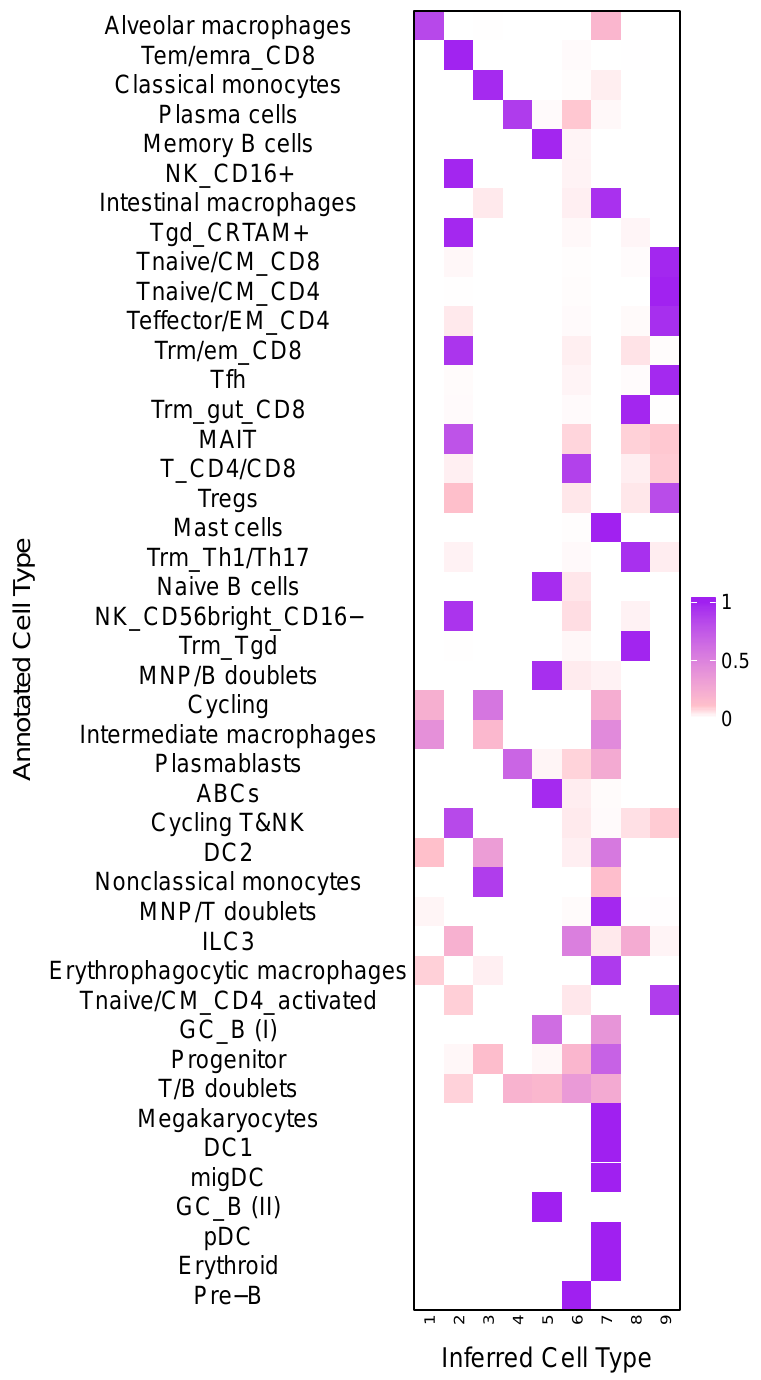
Next, generate a heatmap that displays how cells from each cell-type (determined by the "true" labels obtained from Domínguez Conde et al 2022) are distributed across clusters that are identified by NCLUSION. Each row, i, represents one cell-type, and each column, j, represents one cluster. Therefore the color intensity at location (i, j) on the heatmap corresponds to percent of cells with "true" cell-type label i that were assigned to cluster j by NCLUSION.

To generate the heatmap from the NCLUSION result, enter the following commands into a bash terminal.

NOTE: be sure to replace --nclusion_results input with the relative path to your NCLUSION clustering results.

NOTE: if you want to load packages from a specific R library, append --rlib="/PATH/TO/R/LIBRARY" onto this command.

. tutorial_scripts/make_heatmap.sh --nclusion_results="/PATH/TO/NCLUSION/CLUSTERING/FILE" --pct_table="dominguezconde2022_outputs/cell_distribution_table.csv" --cluster_dict="tutorial_scripts/cluster_mapping/dominguezconde_mapping.csv" --save_heatmap="dominguezconde2022_outputs/cell_distribution_heatmap.pdf" --data_name="dominguezconde"

This will produce a pdf file named dominguezconde2022_outputs/cell_distriubtion_heatmap.pdfcontaining the cell distriubtion heatmap shown below. The column labels do not correspond to NCLUSION's cluster labels. The script labels each cluster with their positional values in the heatmap for aesthetic purposes. A mapping of the original NCLUSION cluster labels to these new positional labels can be found in a file named tutorial_scripts/cluster_mapping/dominguezconde_mapping.csv

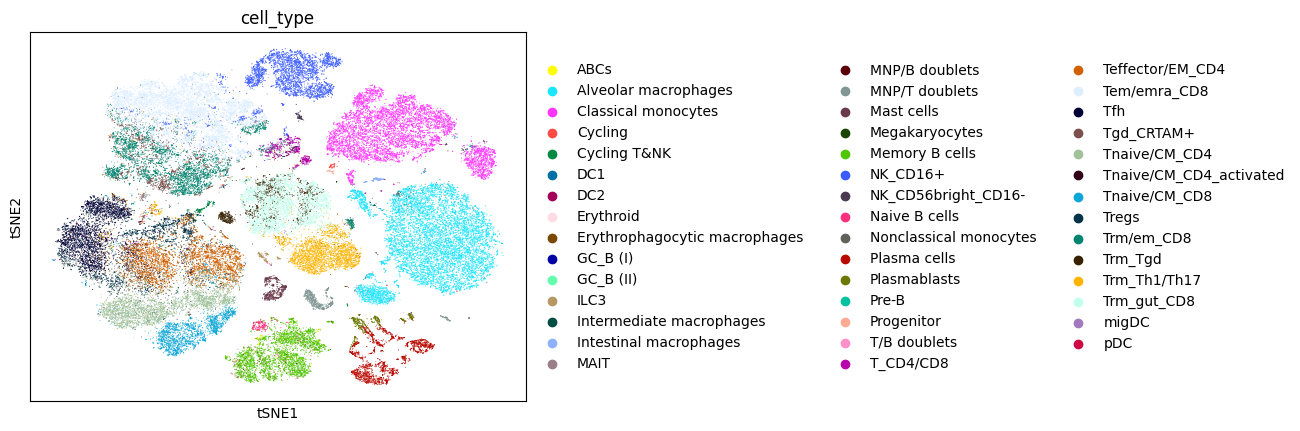
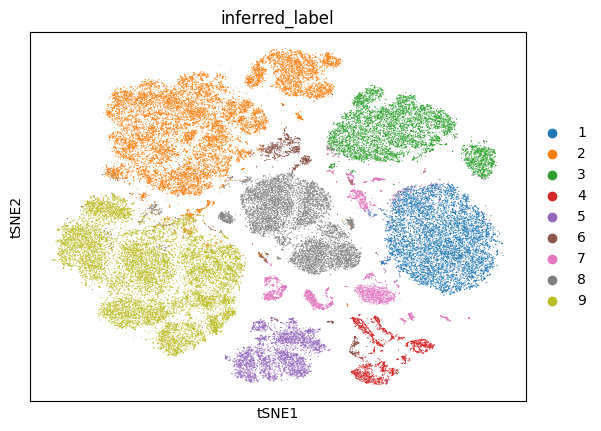
C. Annotated TSNEs

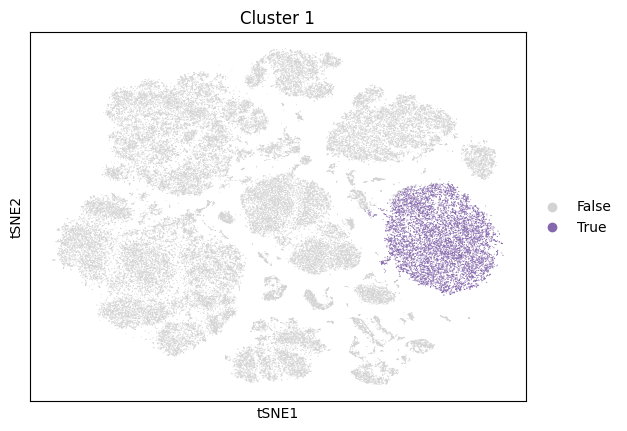
Now, we will plot the t-distributed stochastic neighbor embedding (tSNE) for the data annotated with various labels: the called cell type labels that were published along with the data, and the NCLUSION-inferred cell type labels. We will also generate tSNEs corresponding to the boolean label of each cells' membership to a given NCLUSION-inferred cluster, such that cells assigned to cluster n are colored and all other cells are greyed out. The total number of tSNEs produced are equal to the total number of NCLUSION-inferred clusters plus two. Run the following command to generate these plots.

NOTE: be sure to replace --nclusion_results input with the relative path to your NCLUSION clustering results.

. tutorial_scripts/make_tsnes.sh --datapath="tutorial_data/dominguezconde2022/5000hvgs_dominguezconde2022_preprocessed.h5ad" --nclusion_results="/PATH/TO/NCLUSION/CLUSTERING/FILE" --data_name="dominguezconde2022"

mv figures/ dominguezconde2022_outputs/

All tsnes produces by this script can be found in the output directory: dominguezconde2022_outputs/figures/. The tSNEs colored by called cell-type, inferred cell-type, and Cluster 1 membership are shown below.

D. Variable Selection Analysis

Next, analyze results of NCLUSION's variable selection functionality to gain insight into the biological mechanisms driving the formation of each cluster. The resulting plots are described in detail in the following sub-sections. To generate these plots, enter the following command into a bash terminal.

NOTE: if you want to load packages from a specific R library, append --rlib="/PATH/TO/R/LIBRARY" onto this command.

NOTE: be sure to replace --nclusion_results, --pips, and --path_to_nk inputs with the relative path to your clustering assignment, PIP, and Nk results files (generated by NCLUSION).

. tutorial_scripts/analyze_results.sh --datapath="tutorial_data/dominguezconde2022/5000hvgs_dominguezconde2022_preprocessed.h5ad" --pips="/PATH/TO/PIPS/FILE" --nclusion_results="/PATH/TO/NCLUSION/CLUSTERING/FILE" --output_dir="dominguezconde2022_outputs/" --data_name='dominguezconde' --mapping="tutorial_scripts/cluster_mapping/dominguezconde_mapping.csv" --path_to_nk="PATH/TO/NK/FILE"

All plots produced by this script can be found in the specified output directory: dominguezconde2022_outputs/ directory. Each plot is described in detail below.

i. Adjusted Posterior Inclusion Probability (PIP) Heatmap

We generated a heatmap that displays adjusted Posterior Inclusion Probabilities (PIPs) of genes across clusters identified by NCLUSION. We use PIPs as a summary of evidence for gene being associated with driving the identity of any phenotypic cluster. For a particular cluster, a higher PIP indicates that a gene is more significant to the formation of that cluster. Before generating this heatmap, the plotting script adjusted the PIP values to account for the number of clusters in which it is deemed significant. For example, if a gene is deemed to be significant in driving all clusters, its PIP score will be scaled down, as it is less helpful for identifying important differences between each cluster compared to unique significant genes that are identified in fewer clusters. Only genes with adjusted PIPs above a threshold of 0.5 are included in this analysis. The plot is saved to dominguezconde2022_outputs/heatmap_AdjustedPips_KbyG_defaultclustering.pdf.

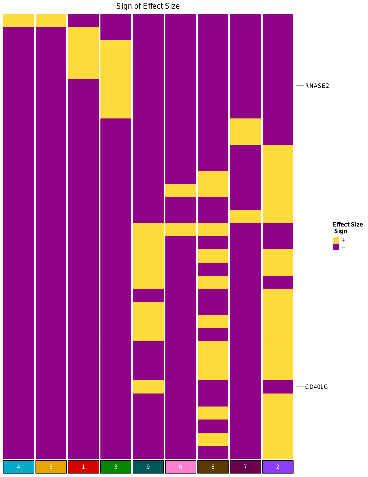
ii. Effect Size Heatmap

The script also generated heatmap representing the effect size of the genes included in the adjusted PIP heatmap, which is shown below. For a given cluster, the effect size indicates the direction of expression (+ or -) for each gene in that cluster. The plot is saved to dominguezconde2022_outputs/heatmap_EffectSizeSignMat_KbyG_basedonAdjPips.pdf

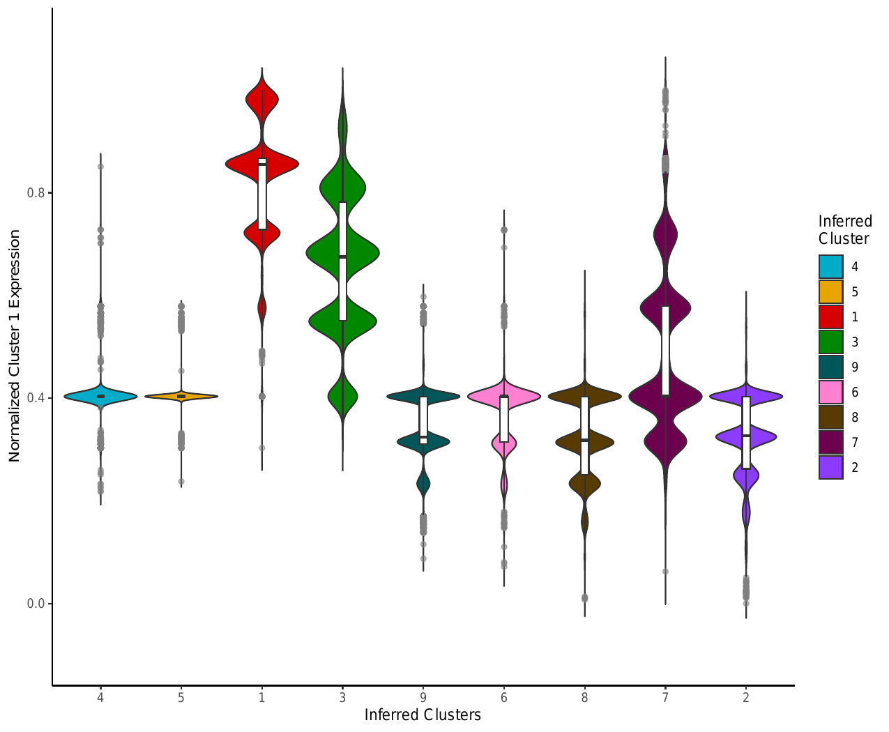
iii. Module Expression Violin Analysis

In addition to the heatmaps, this script generated module expression violin plots for each cluster. Each violin plot compares the expression of significant genes identified in a particular cluster to the expression of that group of genes in the other clusters. The module expression analysis for Cluster 1 is shown below. The plots are saved to dominguezconde2022_outputs/violinplot_tsne_normedmodulescore_colored_nolegend_Cluster_NGenes.pdf where N is equal to the cluster label.

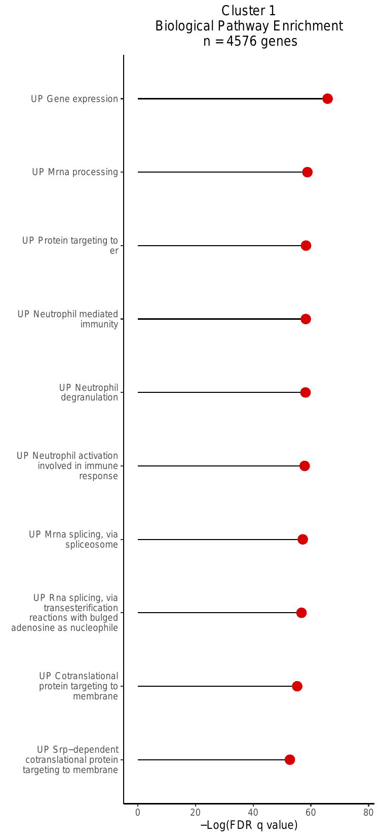
v. Gene-set Over-Enrichment (GO) Analysis

Lastly, this script produced biological pathway enrichment plots. For each cluster, this analysis uses a hypergeometric test to calculate the enrichment of genes in a supplied gene set (genes with significant PIPs [>0.5] in that cluster). The GO analysis for Cluster 1 is shown below. The plots are saved to dominguezconde2022_outputs/GO_bp_enrichmentplots_Cluster_NGenes.pdf where N is equal to the cluster label.

References

C. Dom ́ınguez Conde, C. Xu, L. B. Jarvis, D. B. Rainbow, S. B. Wells, T. Gomes, S. K. Howlett, O. Suchanek, K. Polanski, H. W. King, L. Mamanova, N. Huang, P. A. Szabo, L. Richardson, L. Bolt, E. S. Fasouli, K. T. Mahbubani, M. Prete, L. Tuck, N. Richoz, Z. K. Tuong, L. Campos, H. S. Mousa, E. J. Needham, S. Pritchard, T. Li, R. Elmentaite, J. Park, E. Rahmani, D. Chen, D. K. Menon, O. A. Bayraktar, L. K. James, K. B. Meyer, N. Yosef, M. R. Clatworthy, P. A. Sims, D. L. Farber, K. Saeb-Parsy, J. L. Jones, and S. A. Teichmann. Cross-tissue immune cell analysis reveals tissue-specific features in humans. Science, 376(6594):eabl5197, May 2022. doi: 10.1126/science.abl5197. https://doi.org/10.1126/science.abl5197↩︎