Plotting a Network Graph using network_p2p

2025-06-17

This script demonstrates how to generate and visualize a network graph using the network_p2p function. The function creates an igraph object, which can be plotted to display connections between individuals based on collaboration metrics.

Step 1: Load libraries and sample data

In this example, we will use the sample p2p_data_sim() dataset from the vivainsights package. We will also use dplyr for data manipulation, igraph for network graph creation, ggplot2 for visualization, and ggraph for enhanced network plotting.

library(igraph)
library(ggplot2)
library(RColorBrewer)
library(ggraph)
library(dplyr)
library(vivainsights)

# Define HR variable
hrvar_text <- "Organization"

# Display the first few rows of the dataset
head(p2p_data_sim())

##   PrimaryCollaborator_PersonId SecondaryCollaborator_PersonId
## 1                     SIM_ID_1                       SIM_ID_2
## 2                     SIM_ID_2                       SIM_ID_3
## 3                     SIM_ID_3                       SIM_ID_4
## 4                     SIM_ID_4                       SIM_ID_5
## 5                     SIM_ID_5                       SIM_ID_6
## 6                     SIM_ID_6                       SIM_ID_7
##   PrimaryCollaborator_Organization SecondaryCollaborator_Organization
## 1                            Org F                              Org F
## 2                            Org F                              Org E
## 3                            Org E                              Org D
## 4                            Org D                              Org C
## 5                            Org C                              Org B
## 6                            Org B                              Org A
##   PrimaryCollaborator_LevelDesignation SecondaryCollaborator_LevelDesignation
## 1                              Level 1                                Level 2
## 2                              Level 2                                Level 3
## 3                              Level 3                                Level 4
## 4                              Level 4                                Level 5
## 5                              Level 5                                Level 6
## 6                              Level 6                                Level 7
##   PrimaryCollaborator_City SecondaryCollaborator_City StrongTieScore
## 1                   City C                     City B              1
## 2                   City B                     City A              1
## 3                   City A                     City B              1
## 4                   City B                     City C              1
## 5                   City C                     City A              1
## 6                   City A                     City C              1

Step 2: Generate the igraph network object

The network_p2p() function constructs a network graph based on collaboration data. We set:

• data to the simulated P2P dataset
• hrvar to define the grouping attribute
• return = "network" to get an igraph object

g <- network_p2p(
  data = p2p_data_sim(), 
  hrvar = hrvar_text, 
  return = "network")

# Ensure g is an igraph object
if (!inherits(g, "igraph")) {
  stop("network_p2p did not return an igraph object. Check function parameters.")
}

Step 3: Prepare and customize the graph for visualization

Before plotting, we refine the graph by:

• Removing loops (self-connections) and multiple edges (redundant links)
• Extracting unique values for color mapping
• Assigning colors and scaling node sizes

# Simplify the graph (remove redundant edges and self-loops)
g <- simplify(g, remove.multiple = TRUE, remove.loops = TRUE)

# Extract unique values for color mapping
unique_values <- unique(V(g)$Organization)
num_unique_values <- length(unique_values)

# Generate a color palette
colors <- brewer.pal(min(num_unique_values, 8), "Set2")
org_to_color <- setNames(colors, unique_values)

# Assign colors and scale node sizes
V(g)$node_color <- org_to_color[V(g)$Organization]
V(g)$node_size <- V(g)$node_size * 120  # Ensure this attribute exists

Step 4: Customize and plot the network graph

We use ggraph to create a visually appealing graph with:

• Edge color → blue
• Vertex color → mapped to organization groups
• Vertex size → scaled according to node_size
• Theme adjustments for a dark background and enhanced readability

ggraph(g, layout = "mds") +
  geom_edge_link(aes(edge_alpha = 0.3), color = "#1f78b4") +
  geom_node_point(aes(size = V(g)$node_size, color = factor(V(g)$Organization))) +  
  scale_color_manual(values = org_to_color) +  
  theme_minimal(base_family = "sans") +  # Use a generic, available font
  theme(
    plot.background = element_rect(fill = "white", color = NA),
    panel.grid = element_blank(),  
    legend.text = element_text(size = 10, color = "black"),
    legend.background = element_rect(fill = "white"),
    legend.key = element_rect(fill = "white")
  ) +
  guides(color = guide_legend(override.aes = list(size = 5)), size = FALSE)

## Warning: The `<scale>` argument of `guides()` cannot be `FALSE`. Use "none" instead as
## of ggplot2 3.3.4.
## This warning is displayed once every 8 hours.
## Call `lifecycle::last_lifecycle_warnings()` to see where this warning was
## generated.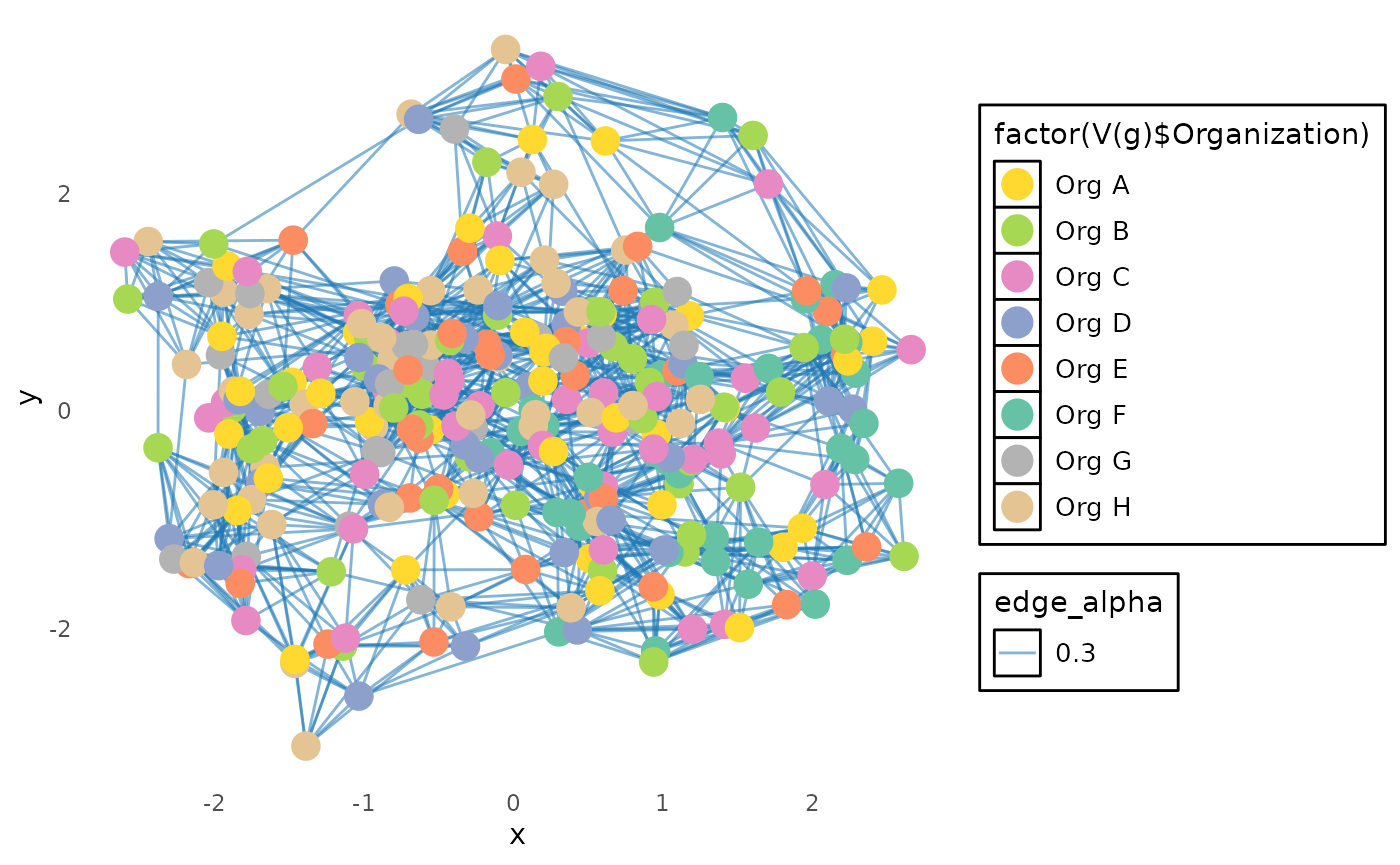

This final plot displays a network of peer-to-peer collaborations based on organization groupings, using a structured and aesthetically refined visualization.