Identifying noteworthy groups with rank functions

Introduction

This article introduces the rank functions that are included in the vivainsights R package. These are powerful functions that scan a full person query dataset and automatically identify noteworthy groups, i.e. those exhibiting the highest or lowest values for a metric in the population.

Rank functions can uncover previously unknown patterns and interesting trends, without analysts having to manually slice the data across multiple attributes. You can think of them as a tool for automatic group exploration - an efficient method for identifying the top and bottom group of employees without manually reviewing all the possible organisational divisions.

Additionally, these functions can reveal what combination of attributes best describe a group that shows a specific behaviour (i.e for example, what organisational attributes represent employees suffering from excessive workload, receiving insufficient coaching, etc). As business leaders often want to develop targeted interventions to address specific issues, these functions can be a great way to inform action planning and transformation initiatives.

This article is divided in four sections. After this introduction, section two describes rank functions and show how them can be used with person query outputs. In the following section, we explore their use for profiling - i.e. to identify in which groups a specific behaviour is most common. The fourth and final section includes a list of additional use cases that can benefit from this method.

Rank Functions

Baseline analysis

To get started, let’s open a new session in R and load the vivainsights R package. We will also use dplyr to facilitate data manipulation:

library(vivainsights)
library(dplyr)

We will use the pq_data demo dataset, which contains a weekly person query output, and apply the collaboration_rank() function:

pq_data %>% 
    collaboration_rank(return = "table")
#> # A tibble: 22 × 4
#>    hrvar            group      Collaboration_hours     n
#>    <chr>            <chr>                    <dbl> <int>
#>  1 FunctionType     Technician                23.6   274
#>  2 Organization     Operations                23.5    22
#>  3 Organization     Research                  23.3    52
#>  4 Level            Level1                    23.2    37
#>  5 LevelDesignation Executive                 23.2    37
#>  6 Organization     HR                        23.1    33
#>  7 Level            Level3                    23.1    87
#>  8 LevelDesignation Senior IC                 23.1    87
#>  9 Organization     Finance                   23.1    68
#> 10 Organization     Sales                     23.1    13
#> # ℹ 12 more rows

The output table contains the results from the automatic group exploration. The rank function has taken all available organisational attributes in this dataset (FunctionType, Organization, LevelDesignation, and IsActive) and calculated the average collaboration hours for each group within each organisational attribute. The table shows the analysed results for all groups, ranked from highest to lowest.

To view the entire table, we can add the function print to the command above.

pq_data %>% 
    collaboration_rank(return = "table") %>%  
    print(n = 30)
#> # A tibble: 22 × 4
#>    hrvar               group          Collaboration_hours     n
#>    <chr>               <chr>                        <dbl> <int>
#>  1 FunctionType        Technician                    23.6   274
#>  2 Organization        Operations                    23.5    22
#>  3 Organization        Research                      23.3    52
#>  4 Level               Level1                        23.2    37
#>  5 LevelDesignation    Executive                     23.2    37
#>  6 Organization        HR                            23.1    33
#>  7 Level               Level3                        23.1    87
#>  8 LevelDesignation    Senior IC                     23.1    87
#>  9 Organization        Finance                       23.1    68
#> 10 Organization        Sales                         23.1    13
#> 11 SupervisorIndicator Manager                       23.0   266
#> 12 FunctionType        Advisor                       23.0   293
#> 13 FunctionType        Consultant                    23.0   288
#> 14 FunctionType        Specialist                    23.0   300
#> 15 FunctionType        Manager                       23.0   300
#> 16 Level               Level4                        22.9   136
#> 17 LevelDesignation    Junior IC                     22.9   136
#> 18 Organization        IT                            22.8    68
#> 19 Level               Level2                        22.8    40
#> 20 LevelDesignation    Senior Manager                22.8    40
#> 21 SupervisorIndicator IC                            22.8    34
#> 22 Organization        Legal                         22.5    44

This analysis shows us that the 82 employees labelled as "FunctionType = "Sales" have the highest collaboration hours, with a weekly average of 31 hours. In second place, there are 60 individuals in Organization = "Inventory Management" with 26.2 hours. On the lower end, the 75 employees labelled as Organization = "Biz Dev" appear to have the lowest collaboration time.

This output is useful to identify groups that are worth investigating (e.g. employees labelled as "FunctionType = Sales"). It also reveals that splits by FunctionType and Organization are more interesting than those by LevelDesignation, as they have more variation; all groups in LevelDesignation have similar levels of collaboration, between 18 and 22 hours a week. 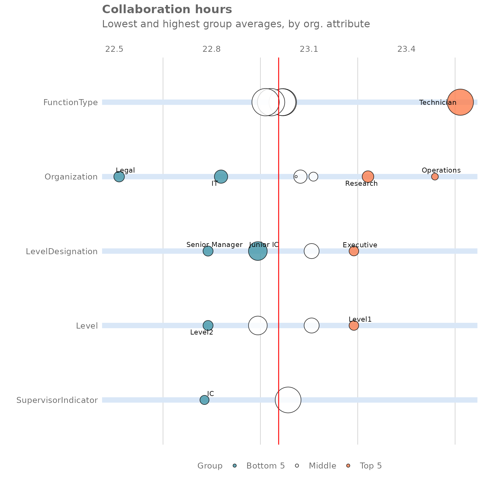Rank functions can also display this information in visual form. We can get that by changing the return argument from "table" to "plot":

pq_data %>% 
    collaboration_rank(return = "plot")

This plot contains the same information as the table above. Each row corresponds to a different organisational attribute and the bubbles show how the population is split across different subgroups, where bubble size is proportional to the number of individuals. The five groups in orange are clearly the ones spending most time in collaboration, with Sales being far ahead of the other groups. Keep in mind that each row of bubbles represents a different way to slice the same population, so groups across rows are not mutually exclusive.

Combining two HR variables

In our baseline analysis, we uncovered that the 82 employees labelled as FunctionType = "Sales" have the highest average collaboration hours. However, it is likely that some employees in this group are more affected than others. Furthermore, there may be pockets in other parts of this company that may be experiencing similar levels of collaboration overload, but that are hidden given the structure of the organisational data (for example, the managers within a particular business unit).

The rank function includes an additional mode called “combine” that allows us to take our analysis one step further by performing on two HR variables the same analysis in a combinatorial manner:

pq_data %>% 
    collaboration_rank(return = "table", mode = "combine")
#> # A tibble: 308 × 4
#>    hrvar    group                                      Collaboration_hours     n
#>    <chr>    <chr>                                                    <dbl> <int>
#>  1 Combined [FunctionType] Technician [SupervisorIndi…                23.8   243
#>  2 Combined [FunctionType] Consultant [SupervisorIndi…                23.1    33
#>  3 Combined [FunctionType] Advisor [SupervisorIndicat…                23.1   260
#>  4 Combined [FunctionType] Manager [SupervisorIndicat…                23.0   266
#>  5 Combined [FunctionType] Consultant [SupervisorIndi…                23.0   255
#>  6 Combined [FunctionType] Specialist [SupervisorIndi…                23.0   266
#>  7 Combined [FunctionType] Specialist [SupervisorIndi…                22.8    34
#>  8 Combined [FunctionType] Advisor [SupervisorIndicat…                22.6    33
#>  9 Combined [FunctionType] Manager [SupervisorIndicat…                22.5    34
#> 10 Combined [FunctionType] Technician [SupervisorIndi…                21.7    31
#> # ℹ 298 more rows

The output table contains similar results from the group exploration above, but with more granularity. The function has automatically created smaller groups by combining two distinct groups from the organisational attributes in scope. In this case, it seems that the 28 managers in Sales are the worst affected group, with a weekly average of 33.7 hours in collaboration per week - that sounds like a lot of meetings!

Additional functions

So far, we have limited our analysis to collaboration_rank(), which only performs the analysis on the metric Collaboration_hours. However, the vivainsights R package includes many other rank functions for key Viva Insights metrics:

afterhours_rank() - for After_hours_collaboration_hours
email_rank() - for Email_hours
meeting_rank() - for Meeting_hours
one2one_rank() - for Meeting_hours_with_manager_1_on_1
workloads_rank() - for Collaboration_span

Additionally, if you want to apply this to any other numeric variable of your choice, you can use the more general version below by specifying the metric as a string with the argument metric:

create_rank()

Using rank functions for profiling

In the previous section, we explored how rank functions can help analysts uncover interesting insights, without the need of manually slicing the data across multiple attributes.

Rank functions have an additional use: they can help us identify what combination of attributes best describe a group that shows a given behaviour. For example, we may be concerned about individuals that are experiencing both a heavy collaboration load (more than 20 hours a week on average) and long workweeks (workweek span of over 60 hours), and would like to know where in the organisations these individuals sit.

To answer that question, let’s create a new numeric custom metric (i.e. a binary flag that is only either 1 or 0) and then apply the create_rank() function:

pq_data %>%
    mutate(At_risk = ifelse(Collaboration_hours > 20 &  Collaboration_span > 60 , 1, 0)) %>%
    create_rank(metric = "At_risk", mode = "combine")
#> # A tibble: 308 × 4
#>    hrvar    group                                                  At_risk     n
#>    <chr>    <chr>                                                    <dbl> <int>
#>  1 Combined [FunctionType] Advisor [SupervisorIndicator] IC              0    33
#>  2 Combined [FunctionType] Advisor [SupervisorIndicator] Manager         0   260
#>  3 Combined [FunctionType] Consultant [SupervisorIndicator] IC           0    33
#>  4 Combined [FunctionType] Consultant [SupervisorIndicator] Manag…       0   255
#>  5 Combined [FunctionType] Manager [SupervisorIndicator] IC              0    34
#>  6 Combined [FunctionType] Manager [SupervisorIndicator] Manager         0   266
#>  7 Combined [FunctionType] Specialist [SupervisorIndicator] IC           0    34
#>  8 Combined [FunctionType] Specialist [SupervisorIndicator] Manag…       0   266
#>  9 Combined [FunctionType] Technician [SupervisorIndicator] IC           0    31
#> 10 Combined [FunctionType] Technician [SupervisorIndicator] Manag…       0   243
#> # ℹ 298 more rows

The custom At_risk variable identifies whether any particular person-week exhibits high collaboration hours and long workweeks. By combining this with create_rank(), the analysis reveals that the combination of heavy collaboration load plus long workweeks is most prevalent among the 13 employees in FunctionType = "Sales" and LevelDesignation = "Junior IC". In other words, the average employee of these groups experience high collaboration load and long workweeks 31% of the time.

Conclusion, use cases and other applications

In this article, we have shown how rank functions can be a powerful tool to both uncover previously unknown patterns and to profile the groups that are experiencing a certain behaviour. In the context of Viva Insights, we see a wide range of applications in the areas of wellbeing, ways of working, and sales excellence. Examples include:

Workload: Identifying groups with excessive collaboration and long workdays
Freedom to disconnect: Identifying groups with always-on behaviours
Coaching: Identifying groups with insufficient coaching and manager time
Exposure: Identifying groups with insufficient skip-level exposure
Isolation: Identifying groups with insufficient cross-team collaboration
Sales performance: Identifying groups with insufficient external collaboration

Feedback

We hope you found this article useful!

If you have any suggestions or feedback, please submit an issue at https://github.com/microsoft/vivainsights/issues.

Carlos Morales-Torrado

2025-06-17