Rank all groups across HR attributes on a selected Viva Insights metric

This function scans a standard Person query output for groups with high levels of a given Viva Insights Metric. Returns a plot by default, with an option to return a table with all groups (across multiple HR attributes) ranked by the specified metric.

Usage

create_rank(
  data,
  metric,
  hrvar = extract_hr(data, exclude_constants = TRUE),
  mingroup = 5,
  return = "table",
  mode = "simple",
  plot_mode = 1
)

Arguments

data

A Standard Person Query dataset in the form of a data frame.

metric

Character string containing the name of the metric, e.g. "Collaboration_hours"

hrvar

String containing the name of the HR Variable by which to split metrics. Defaults to "Organization". To run the analysis on the total instead of splitting by an HR attribute, supply NULL (without quotes).

mingroup

Numeric value setting the privacy threshold / minimum group size. Defaults to 5.

return

String specifying what to return. This must be one of the following strings:

"plot" (default)
"table"

See Value for more information.

mode

String to specify calculation mode. Must be either:

"simple"
"combine"

plot_mode

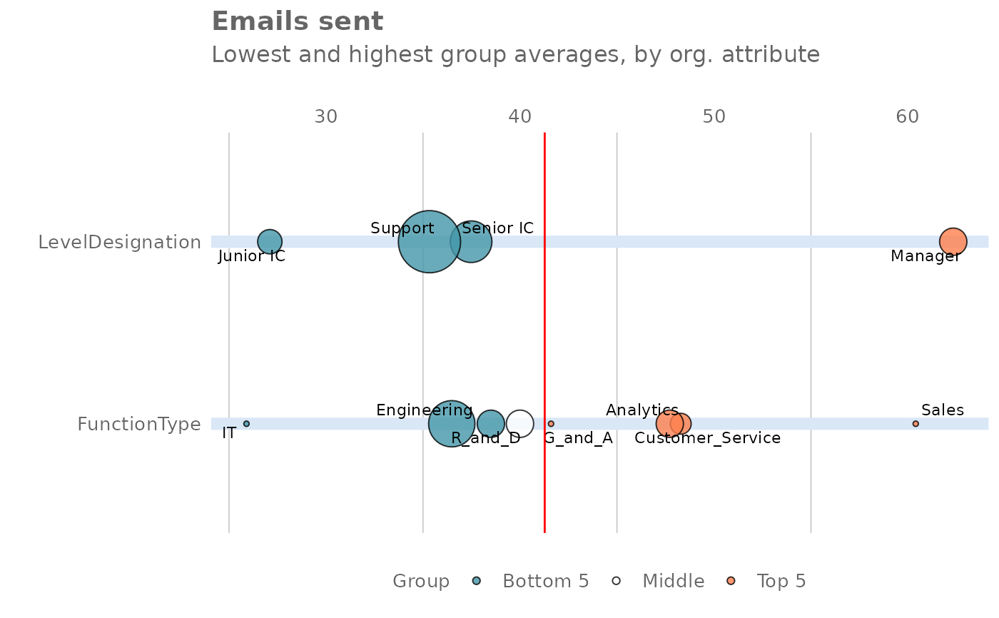
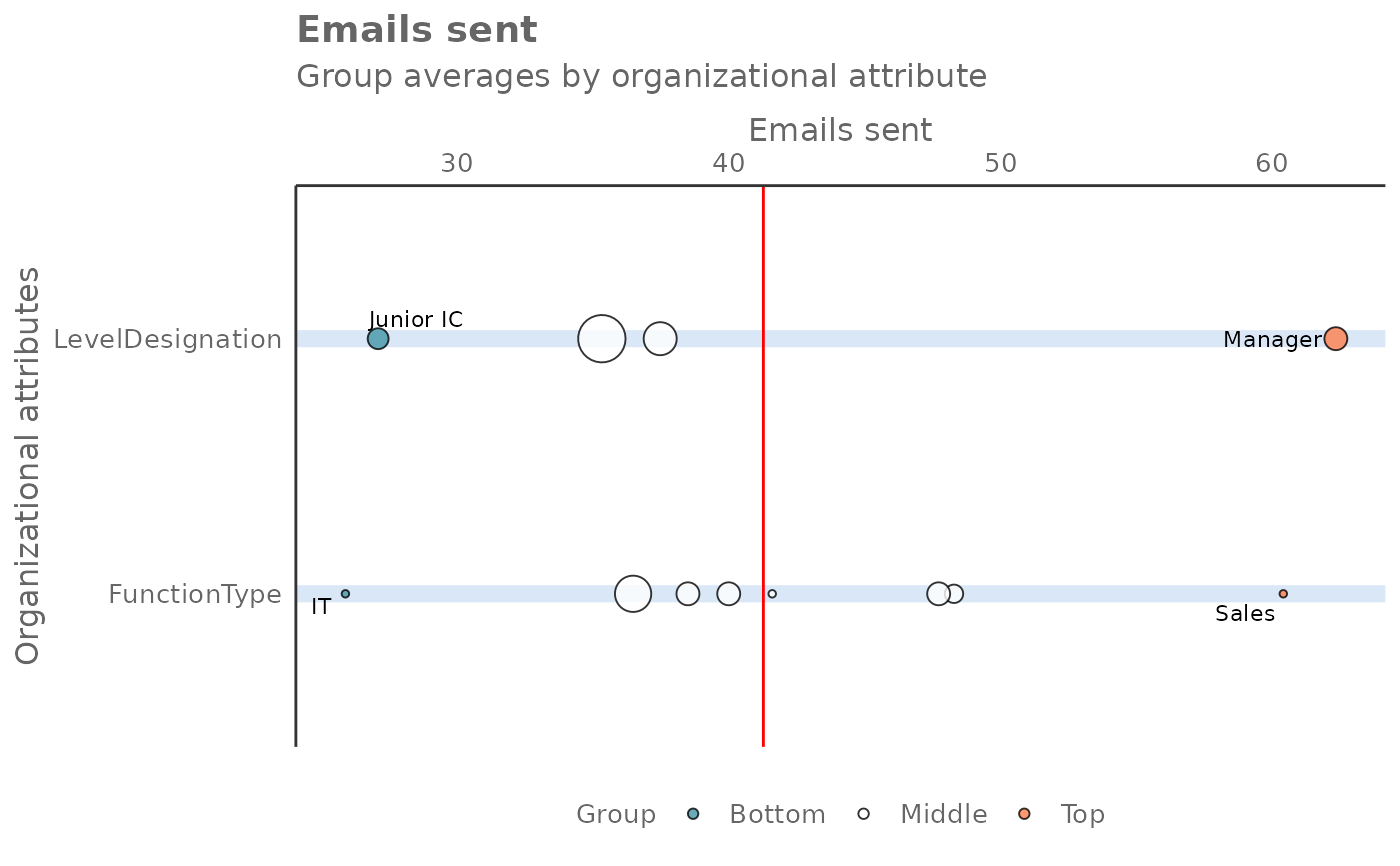
Numeric vector to determine which plot mode to return. Must be either 1 or 2, and is only used when return = "plot".

1: Top and bottom five groups across the data population are highlighted
2: Top and bottom groups per organizational attribute are highlighted

Value

A different output is returned depending on the value passed to the return argument:

"plot": 'ggplot' object. A bubble plot where the x-axis represents the metric, the y-axis represents the HR attributes, and the size of the bubbles represent the size of the organizations. Note that there is no plot output if mode is set to "combine".
"table": data frame. A summary table for the metric.

Other Visualization: afterhours_dist(), afterhours_fizz(), afterhours_line(), afterhours_rank(), afterhours_summary(), afterhours_trend(), collaboration_area(), collaboration_dist(), collaboration_fizz(), collaboration_line(), collaboration_rank(), collaboration_sum(), collaboration_trend(), create_bar(), create_bar_asis(), create_boxplot(), create_bubble(), create_dist(), create_fizz(), create_inc(), create_line(), create_line_asis(), create_period_scatter(), create_sankey(), create_scatter(), create_stacked(), create_tracking(), create_trend(), email_dist(), email_fizz(), email_line(), email_rank(), email_summary(), email_trend(), external_dist(), external_fizz(), external_line(), external_rank(), external_sum(), hr_trend(), hrvar_count(), hrvar_trend(), keymetrics_scan(), meeting_dist(), meeting_fizz(), meeting_line(), meeting_rank(), meeting_summary(), meeting_trend(), one2one_dist(), one2one_fizz(), one2one_freq(), one2one_line(), one2one_rank(), one2one_sum(), one2one_trend()

Other Flexible: create_bar(), create_bar_asis(), create_boxplot(), create_bubble(), create_density(), create_dist(), create_fizz(), create_hist(), create_inc(), create_line(), create_line_asis(), create_period_scatter(), create_sankey(), create_scatter(), create_stacked(), create_tracking(), create_trend()

Author

Carlos Morales Torrado carlos.morales@microsoft.com

Martin Chan martin.chan@microsoft.com

Examples

pq_data_small <- dplyr::slice_sample(pq_data, prop = 0.1)

# Plot mode 1 - show top and bottom five groups
create_rank(
  data = pq_data_small,
  hrvar = c("FunctionType", "LevelDesignation"),
  metric = "Emails_sent",
  return = "plot",
  plot_mode = 1
)


# Plot mode 2 - show top and bottom groups per HR variable
create_rank(
  data = pq_data_small,
  hrvar = c("FunctionType", "LevelDesignation"),
  metric = "Emails_sent",
  return = "plot",
  plot_mode = 2
)


# Return a table
create_rank(
  data = pq_data_small,
  metric = "Emails_sent",
  return = "table"
)
#> # A tibble: 22 × 4
#>    hrvar               group     Emails_sent     n
#>    <chr>               <chr>           <dbl> <int>
#>  1 FunctionType        Advisor          45.8    83
#>  2 Organization        IT               45.3    61
#>  3 Organization        Research         44.7    46
#>  4 FunctionType        Manager          44.5   140
#>  5 Level               Level4           44.3   126
#>  6 LevelDesignation    Junior IC        44.3   126
#>  7 SupervisorIndicator IC               44.3    32
#>  8 Organization        Finance          44.0    65
#>  9 SupervisorIndicator Manager          43.7   247
#> 10 Level               Level3           43.7    84
#> # ℹ 12 more rows

# \donttest{
# Return a table - combination mode
create_rank(
  data = pq_data_small,
  metric = "Emails_sent",
  mode = "combine",
  return = "table"
)
#> # A tibble: 296 × 4
#>    hrvar    group                                              Emails_sent     n
#>    <chr>    <chr>                                                    <dbl> <int>
#>  1 Combined [FunctionType] Advisor [SupervisorIndicator] IC           52.3     8
#>  2 Combined [FunctionType] Manager [SupervisorIndicator] IC           49.5    19
#>  3 Combined [FunctionType] Advisor [SupervisorIndicator] Mana…        45.1    75
#>  4 Combined [FunctionType] Specialist [SupervisorIndicator] M…        43.8   146
#>  5 Combined [FunctionType] Manager [SupervisorIndicator] Mana…        43.7   121
#>  6 Combined [FunctionType] Consultant [SupervisorIndicator] M…        43.4    77
#>  7 Combined [FunctionType] Technician [SupervisorIndicator] M…        43.0    45
#>  8 Combined [FunctionType] Technician [SupervisorIndicator] IC        42.7     6
#>  9 Combined [FunctionType] Consultant [SupervisorIndicator] IC        40      11
#> 10 Combined [FunctionType] Specialist [SupervisorIndicator] IC        39.2    23
#> # ℹ 286 more rows
# }