Period comparison scatter plot for any two metrics
Source:R/create_period_scatter.R
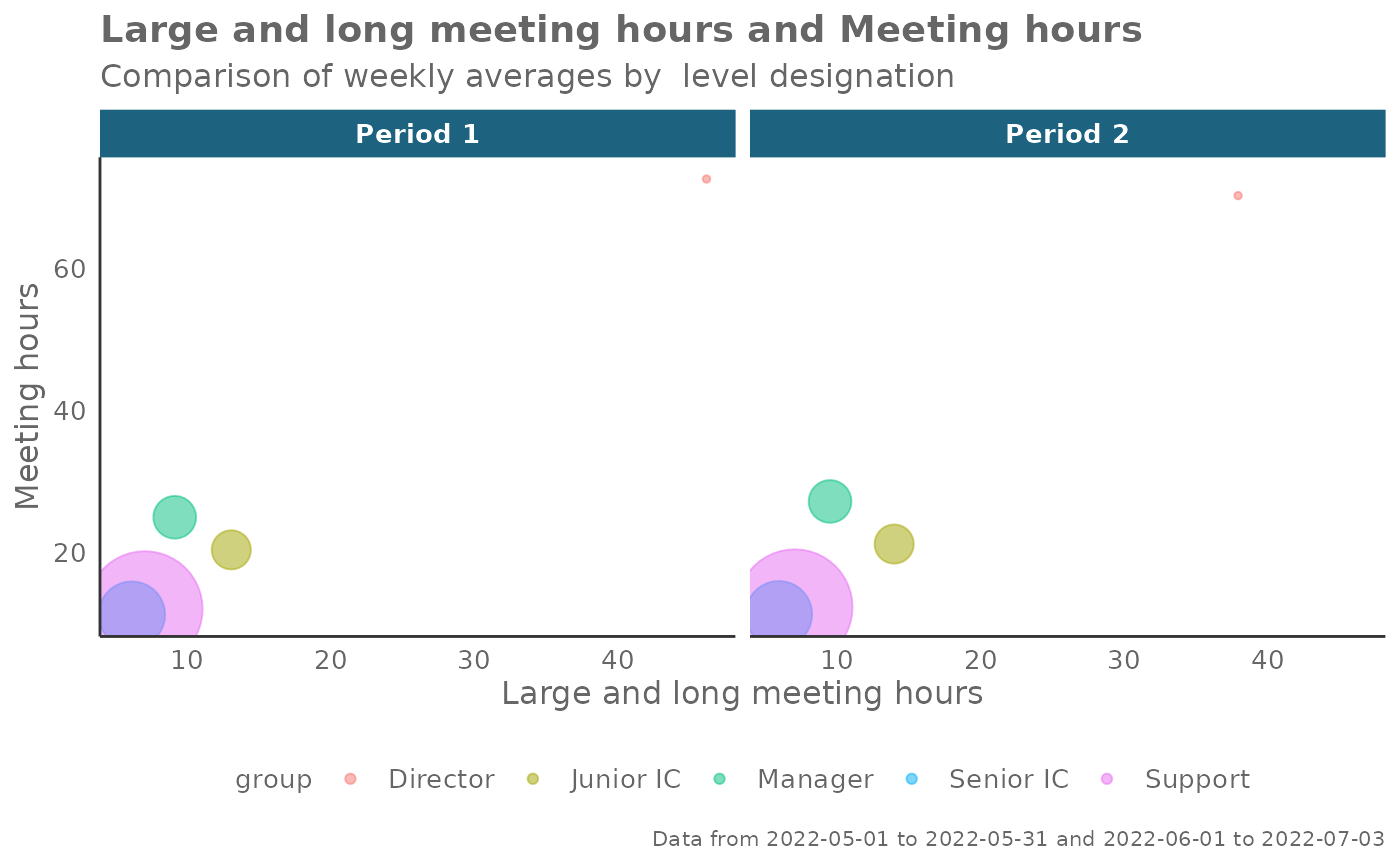
create_period_scatter.RdReturns two side-by-side scatter plots representing two selected metrics, using colour to map an HR attribute and size to represent number of employees. Returns a faceted scatter plot by default, with additional options to return a summary table.
Usage
create_period_scatter(
  data,
  hrvar = "Organization",
  metric_x = "Large_and_long_meeting_hours",
  metric_y = "Meeting_hours",
  before_start = min(as.Date(data$MetricDate, "%m/%d/%Y")),
  before_end,
  after_start = as.Date(before_end) + 1,
  after_end = max(as.Date(data$MetricDate, "%m/%d/%Y")),
  before_label = "Period 1",
  after_label = "Period 2",
  mingroup = 5,
  return = "plot"
)
Arguments
- data
A Standard Person Query dataset in the form of a data frame. This must be a panel dataset where each row represents one employee per time period, with the columns
PersonIdandMetricDatepresent.- hrvar
HR Variable by which to split metrics. Accepts a character vector, defaults to "Organization" but accepts any character vector, e.g. "LevelDesignation"
- metric_x
Character string containing the name of the metric, e.g. "Collaboration_hours"
- metric_y
Character string containing the name of the metric, e.g. "Collaboration_hours"
- before_start
Start date of "before" time period in YYYY-MM-DD
- before_end
End date of "before" time period in YYYY-MM-DD
- after_start
Start date of "after" time period in YYYY-MM-DD
- after_end
End date of "after" time period in YYYY-MM-DD
- before_label
String to specify a label for the "before" period. Defaults to "Period 1".
- after_label
String to specify a label for the "after" period. Defaults to "Period 2".
- mingroup
Numeric value setting the privacy threshold / minimum group size. Defaults to 5.
- return
Character vector specifying what to return, defaults to "plot". Valid inputs are "plot" and "table".
Value
Returns a 'ggplot' object showing two scatter plots side by side representing the two periods.
Details
This is a general purpose function that powers all the functions in the package that produce faceted scatter plots.
See also
Other Visualization:
afterhours_dist(),
afterhours_fizz(),
afterhours_line(),
afterhours_rank(),
afterhours_summary(),
afterhours_trend(),
collaboration_area(),
collaboration_dist(),
collaboration_fizz(),
collaboration_line(),
collaboration_rank(),
collaboration_sum(),
collaboration_trend(),
create_bar(),
create_bar_asis(),
create_boxplot(),
create_bubble(),
create_dist(),
create_fizz(),
create_inc(),
create_line(),
create_line_asis(),
create_radar(),
create_rank(),
create_rogers(),
create_sankey(),
create_scatter(),
create_stacked(),
create_survival(),
create_tracking(),
create_trend(),
email_dist(),
email_fizz(),
email_line(),
email_rank(),
email_summary(),
email_trend(),
external_dist(),
external_fizz(),
external_line(),
external_rank(),
external_sum(),
hr_trend(),
hrvar_count(),
hrvar_trend(),
keymetrics_scan(),
meeting_dist(),
meeting_fizz(),
meeting_line(),
meeting_rank(),
meeting_summary(),
meeting_trend(),
one2one_dist(),
one2one_fizz(),
one2one_freq(),
one2one_line(),
one2one_rank(),
one2one_sum(),
one2one_trend()
Other Flexible:
create_bar(),
create_bar_asis(),
create_boxplot(),
create_bubble(),
create_density(),
create_dist(),
create_fizz(),
create_hist(),
create_inc(),
create_line(),
create_line_asis(),
create_radar(),
create_rank(),
create_sankey(),
create_scatter(),
create_stacked(),
create_survival(),
create_tracking(),
create_trend()
Other Time-series:
create_line(),
create_line_asis(),
create_trend()
Examples
# Return plot
create_period_scatter(pq_data,
                      hrvar = "LevelDesignation",
                      before_start = "2024-05-01",
                      before_end = "2024-05-31",
                      after_start = "2024-06-01",
                      after_end = "2024-07-03")


# Return a summary table
create_period_scatter(pq_data, before_end = "2024-05-31", return = "table")
#> # A tibble: 14 × 5
#>    group      Large_and_long_meeting_hours Meeting_hours Period       n
#>    <chr>                             <dbl>         <dbl> <chr>    <int>
#>  1 Finance                            1.09          18.3 Period 1    68
#>  2 HR                                 1.08          18.4 Period 1    33
#>  3 IT                                 1.02          17.2 Period 1    68
#>  4 Legal                              1.12          22.3 Period 1    44
#>  5 Operations                         1.19          20.5 Period 1    22
#>  6 Research                           1.12          20.6 Period 1    52
#>  7 Sales                              1.13          19.4 Period 1    13
#>  8 Finance                            1.16          19.1 Period 2    68
#>  9 HR                                 1.17          18.3 Period 2    33
#> 10 IT                                 1.11          17.7 Period 2    68
#> 11 Legal                              1.06          16.9 Period 2    44
#> 12 Operations                         1.11          19.6 Period 2    22
#> 13 Research                           1.18          20.1 Period 2    52
#> 14 Sales                              1.11          18.8 Period 2    13
# Return a summary table
create_period_scatter(pq_data, before_end = "2024-05-31", return = "table")
#> # A tibble: 14 × 5
#> group Large_and_long_meeting_hours Meeting_hours Period n
#> <chr> <dbl> <dbl> <chr> <int>
#> 1 Finance 1.09 18.3 Period 1 68
#> 2 HR 1.08 18.4 Period 1 33
#> 3 IT 1.02 17.2 Period 1 68
#> 4 Legal 1.12 22.3 Period 1 44
#> 5 Operations 1.19 20.5 Period 1 22
#> 6 Research 1.12 20.6 Period 1 52
#> 7 Sales 1.13 19.4 Period 1 13
#> 8 Finance 1.16 19.1 Period 2 68
#> 9 HR 1.17 18.3 Period 2 33
#> 10 IT 1.11 17.7 Period 2 68
#> 11 Legal 1.06 16.9 Period 2 44
#> 12 Operations 1.11 19.6 Period 2 22
#> 13 Research 1.18 20.1 Period 2 52
#> 14 Sales 1.11 18.8 Period 2 13