Frequency of Manager 1:1 Meetings as bar or 100% stacked bar chart

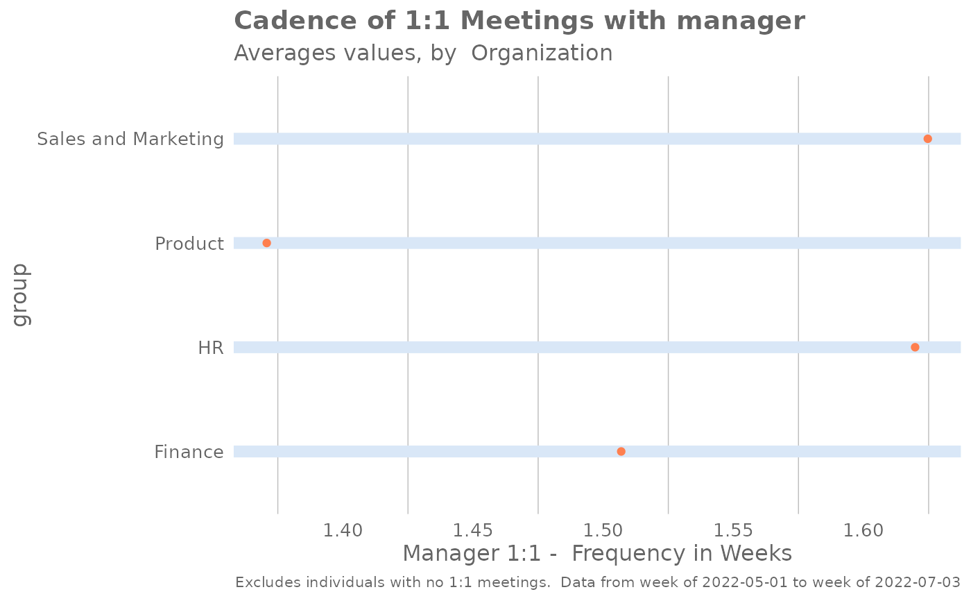
This function calculates the average number of weeks (cadence) between of 1:1 meetings between an employee and their manager. Returns a distribution plot for typical cadence of 1:1 meetings. Additional options available to return a bar plot, tables, or a data frame with a cadence of 1 on 1 meetings metric.

Usage

one2one_freq(
  data,
  hrvar = "Organization",
  mingroup = 5,
  return = "plot",
  mode = "dist",
  sort_by = NULL
)

Arguments

data

A Standard Person Query dataset in the form of a data frame.

hrvar

String containing the name of the HR Variable by which to split metrics. Defaults to "Organization". To run the analysis on the total instead of splitting by an HR attribute, supply NULL (without quotes).

mingroup

Numeric value setting the privacy threshold / minimum group size. Defaults to 5.

return

String specifying what to return. This must be one of the following strings:

"plot"
"table"

mode

String specifying what method to use. This must be one of the following strings:

"dist"
"sum"

sort_by

String to specify the bucket label to sort by. Defaults to NULL (no sorting).

Value

A different output is returned depending on the value passed to the return argument:

"plot": 'ggplot' object. A stacked bar plot for the metric.
"table": data frame. A summary table for the metric.

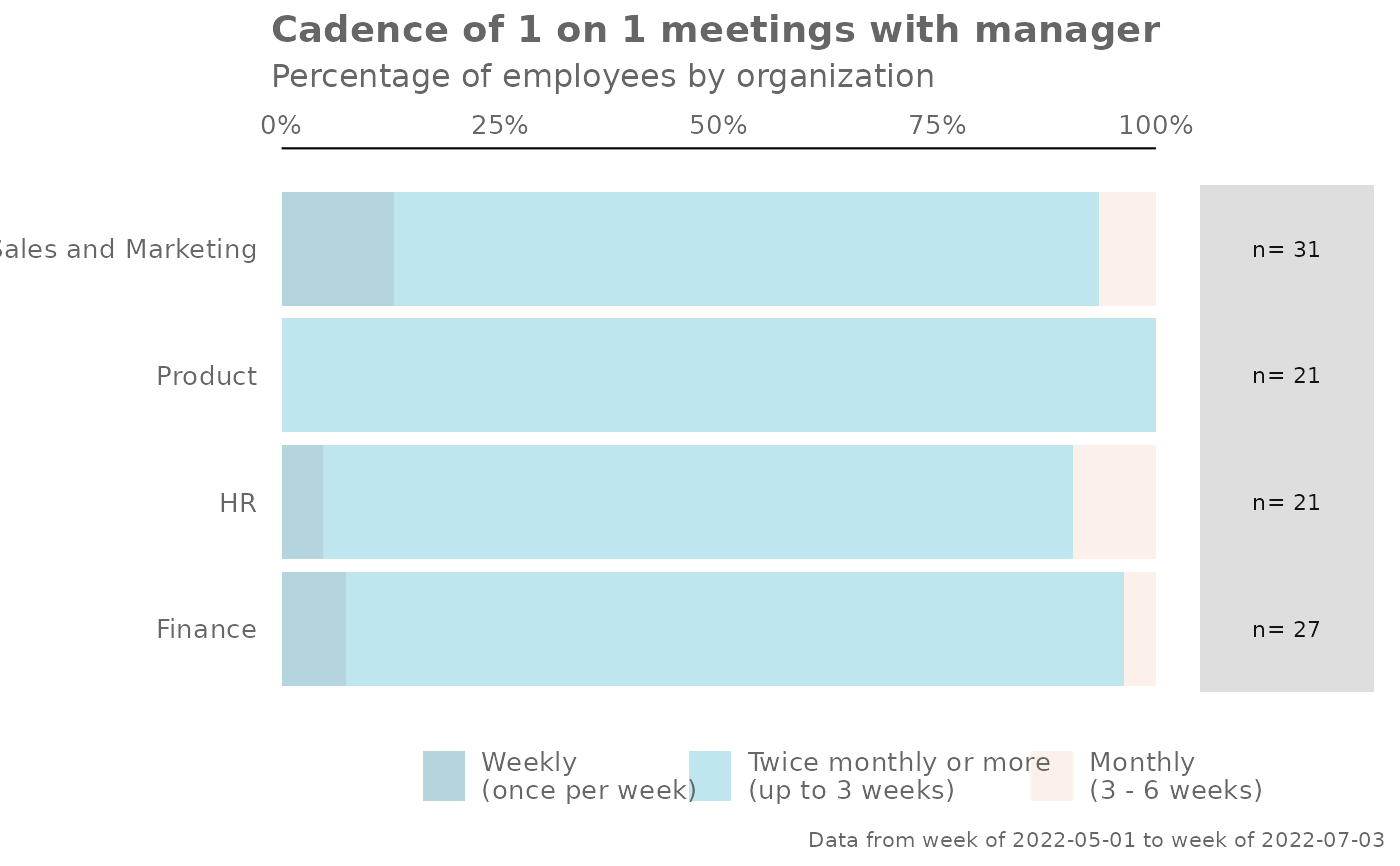
Distribution view

For this view, there are four categories of cadence:

Weekly (once per week)
Twice monthly or more (up to 3 weeks)
Monthly (3 - 6 weeks)
Every two months (6 - 10 weeks)
Quarterly or less (> 10 weeks)

In the occasion there are zero 1:1 meetings with managers, this is included into the last category, i.e. 'Quarterly or less'. Note that when mode is set to "sum", these rows are simply excluded from the calculation.

Other Visualization: afterhours_dist(), afterhours_fizz(), afterhours_line(), afterhours_rank(), afterhours_summary(), afterhours_trend(), collaboration_area(), collaboration_dist(), collaboration_fizz(), collaboration_line(), collaboration_rank(), collaboration_sum(), collaboration_trend(), create_bar(), create_bar_asis(), create_boxplot(), create_bubble(), create_dist(), create_fizz(), create_inc(), create_line(), create_line_asis(), create_period_scatter(), create_rank(), create_rogers(), create_sankey(), create_scatter(), create_stacked(), create_tracking(), create_trend(), email_dist(), email_fizz(), email_line(), email_rank(), email_summary(), email_trend(), external_dist(), external_fizz(), external_line(), external_rank(), external_sum(), hr_trend(), hrvar_count(), hrvar_trend(), keymetrics_scan(), meeting_dist(), meeting_fizz(), meeting_line(), meeting_rank(), meeting_summary(), meeting_trend(), one2one_dist(), one2one_fizz(), one2one_line(), one2one_rank(), one2one_sum(), one2one_trend()

Other Managerial Relations: one2one_dist(), one2one_fizz(), one2one_line(), one2one_rank(), one2one_sum(), one2one_trend()

Examples

# Return plot, mode dist
one2one_freq(pq_data, hrvar = "Organization", return = "plot", mode = "dist")


# Return plot, mode sum
one2one_freq(pq_data,
             hrvar = "Organization",
             return = "plot",
             mode = "sum")


# Return summary table
one2one_freq(pq_data, hrvar = "Organization", return = "table")
#> # A tibble: 7 × 3
#>   group      `Weekly\n(once per week)` Employee_Count
#>   <fct>                          <dbl>          <int>
#> 1 Finance                            1             68
#> 2 HR                                 1             33
#> 3 IT                                 1             68
#> 4 Legal                              1             44
#> 5 Operations                         1             22
#> 6 Research                           1             52
#> 7 Sales                              1             13