Damage Mapping with a Trained Model#
Goal: produce a wall-to-wall damage map. You draw labels on a small area, train a segmentation model on them, and HASTE runs that model across the entire image layer to generate a continuous damage prediction you can visualize and download as a geopackage.
For a faster, building-level result with no training job, see Rapid Building Assessment.
The workflow at a glance
Standard-workflow layer → Label a training area → Train a model → View & export the results.
Before you start#
Create a project and add a Standard-workflow image layer with your pre-/post-event imagery. See Projects and Image layers.
Try it with sample data
New to HASTE? Use the Lahaina, Maui sample (Vantor post-event imagery) from
Image layers (see Sample data to try HASTE): create a
Standard-workflow layer with maxar_lahaina_8_12_2023-visual.tif as the post-event
imagery. Building footprints download automatically from Overture Maps.
Step 1 — Label a training area#
Labeling means manually annotating damaged, undamaged, and background areas on a small section of the imagery. These labels train the model, which then predicts damage across the rest of the image. This step is required before training.
Launch the tool from the Projects page by clicking Launch next to the image layer.
Draw labels#

Use the Pan, Polygon, Rectangle, Circle, Edit, and Delete tools to annotate. Then pick a label class:
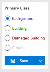
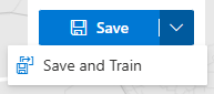
You must select both a tool and a class to draw a label. Click Save to store your labels, or the arrow next to Save to save and start training in one step.
Adjust the imagery#
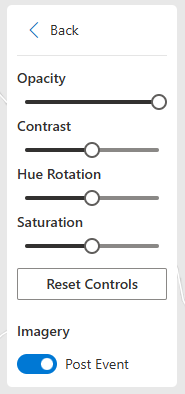
To make damage easier to see while you label, tune the view of the pre-/post-event imagery:
Opacity, Contrast, Hue Rotation, and Saturation sliders (with Reset).
Toggle between post- and pre-event imagery with the imagery switch. Press A for pre-event
(or the Azure Basemap fallback) and D for post-event imagery.
Tips for effective labeling#
The quality of your labels drives the quality of the model. A few pointers:
Minimum number of labels — draw at least 5–10 per class. Training improves with more quality labels; 70–100 make a good training set, and more than ~150 isn’t necessary.
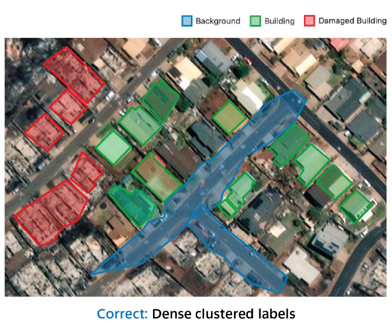
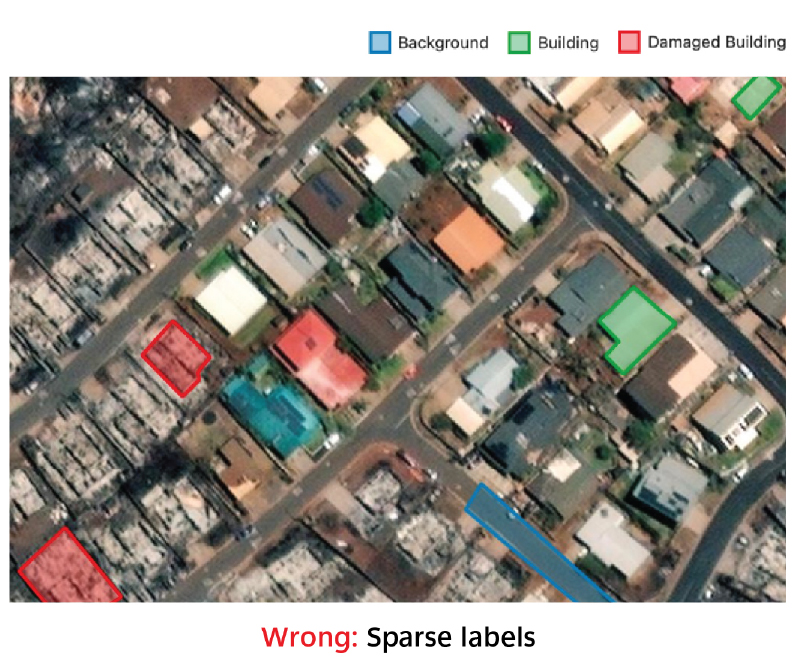
Cluster labels closely — label features adjacent to each other (e.g. a building and the background around it). Unlabeled areas aren’t used in training, so labeling a building without its surroundings lets the model make a blurry prediction without penalty.
Correct |
Incorrect |
|---|---|
|
|
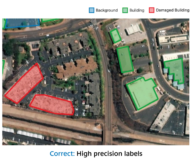
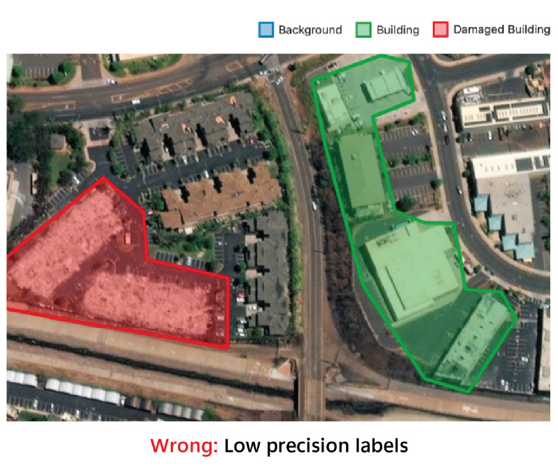
Draw labels precisely — high precision matters more than covering large areas quickly.
Correct |
Incorrect |
|---|---|
|
|
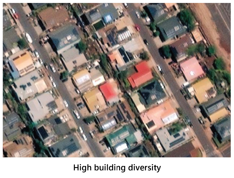
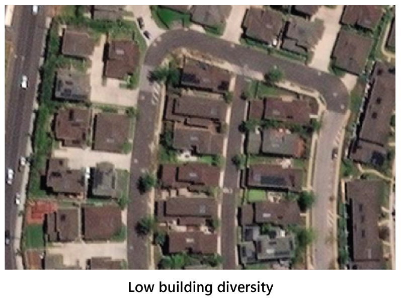
Maximize label diversity — 20 buildings with varied roofs, sizes, and textures teach the model more than 20 identical ones.
High diversity |
Low diversity |
|---|---|
|
|
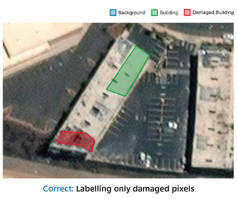
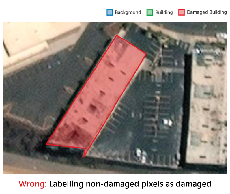
Label relevant portions only — for a partially damaged building, label only the damaged pixels as damaged, not the whole building.
Correct |
Incorrect |
|---|---|
|
|
Step 2 — Train the model#
Satellite imagery varies a lot between regions, so HASTE trains a fresh model on your labels for each run rather than reusing weights across areas. Once you’ve labeled, start training in either of two ways:
Click Save and Train in the labeling tool.
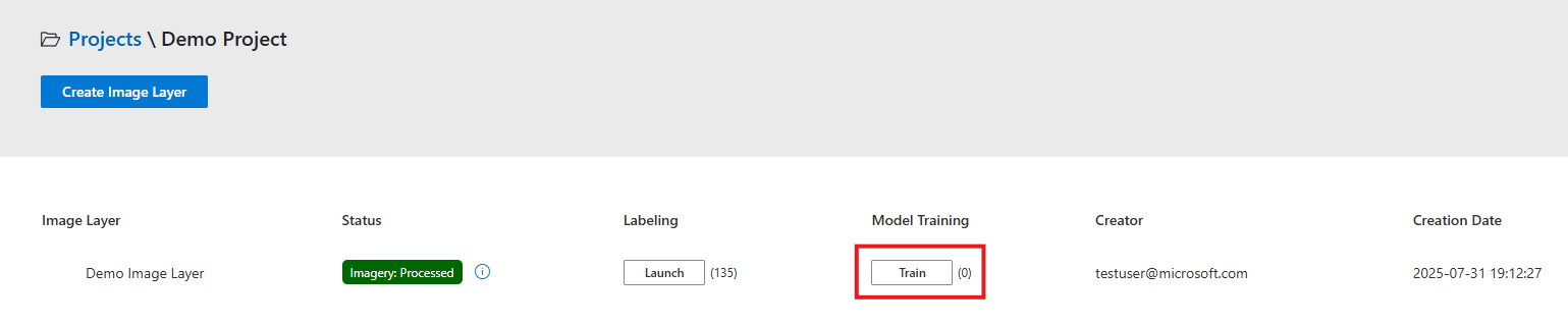
Or click Train for that image layer on the Projects page.
Training parameters#
Leave these at their defaults if you’re unsure:
Model Name — a unique name for your model.
Base Model — a model from the Model catalog to fine-tune. Only models whose event type and imagery source match your layer are shown.
Learning Rate — how much the model adjusts per update.
Batch Size — training examples per iteration; larger is faster but needs more memory.
Max Epochs — passes over the training data.
Step 3 — View and export results#
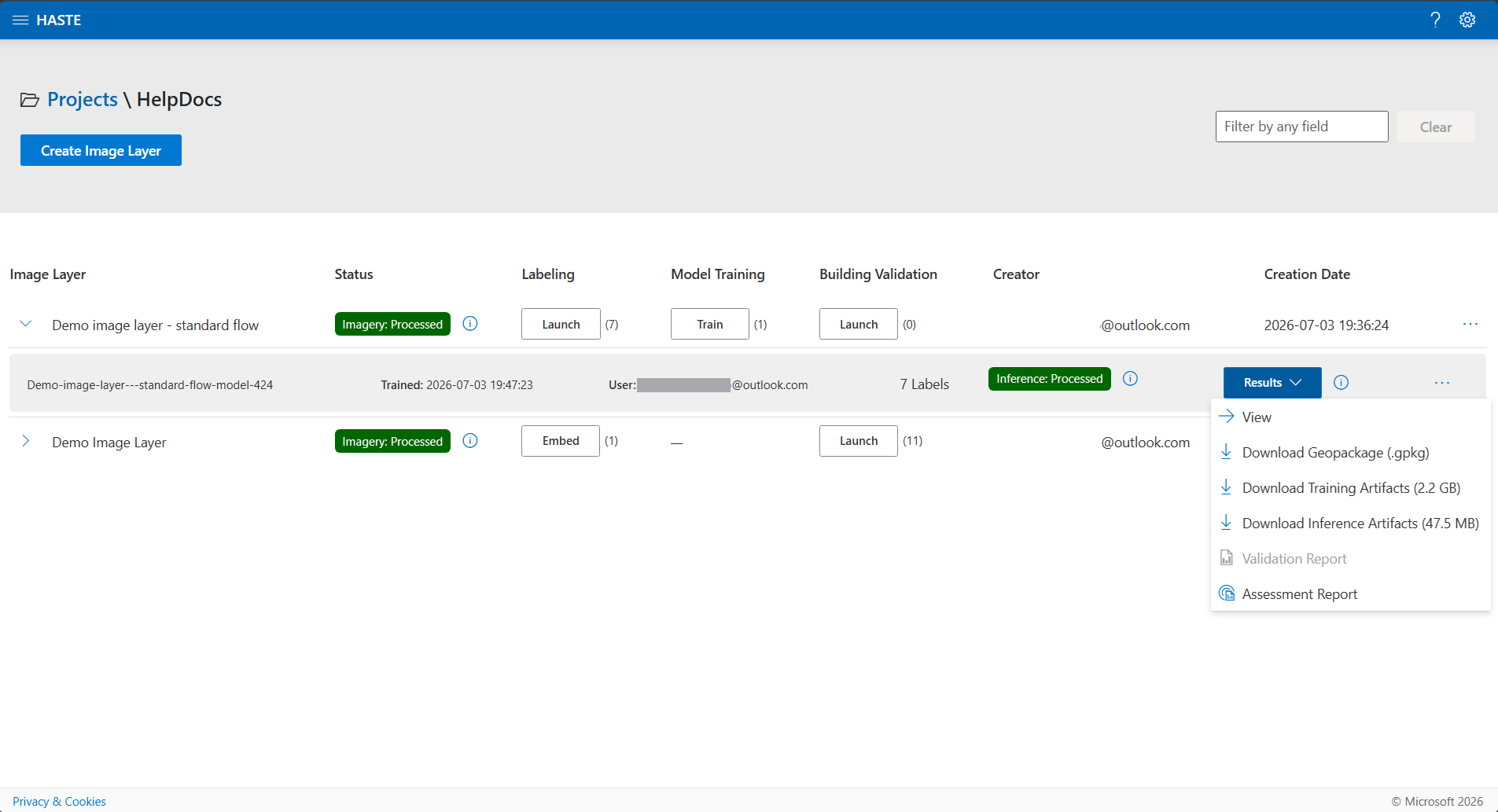
When training and inference finish, open the model’s Results menu for several ways to use the predictions.
View (built-in visualizer)#
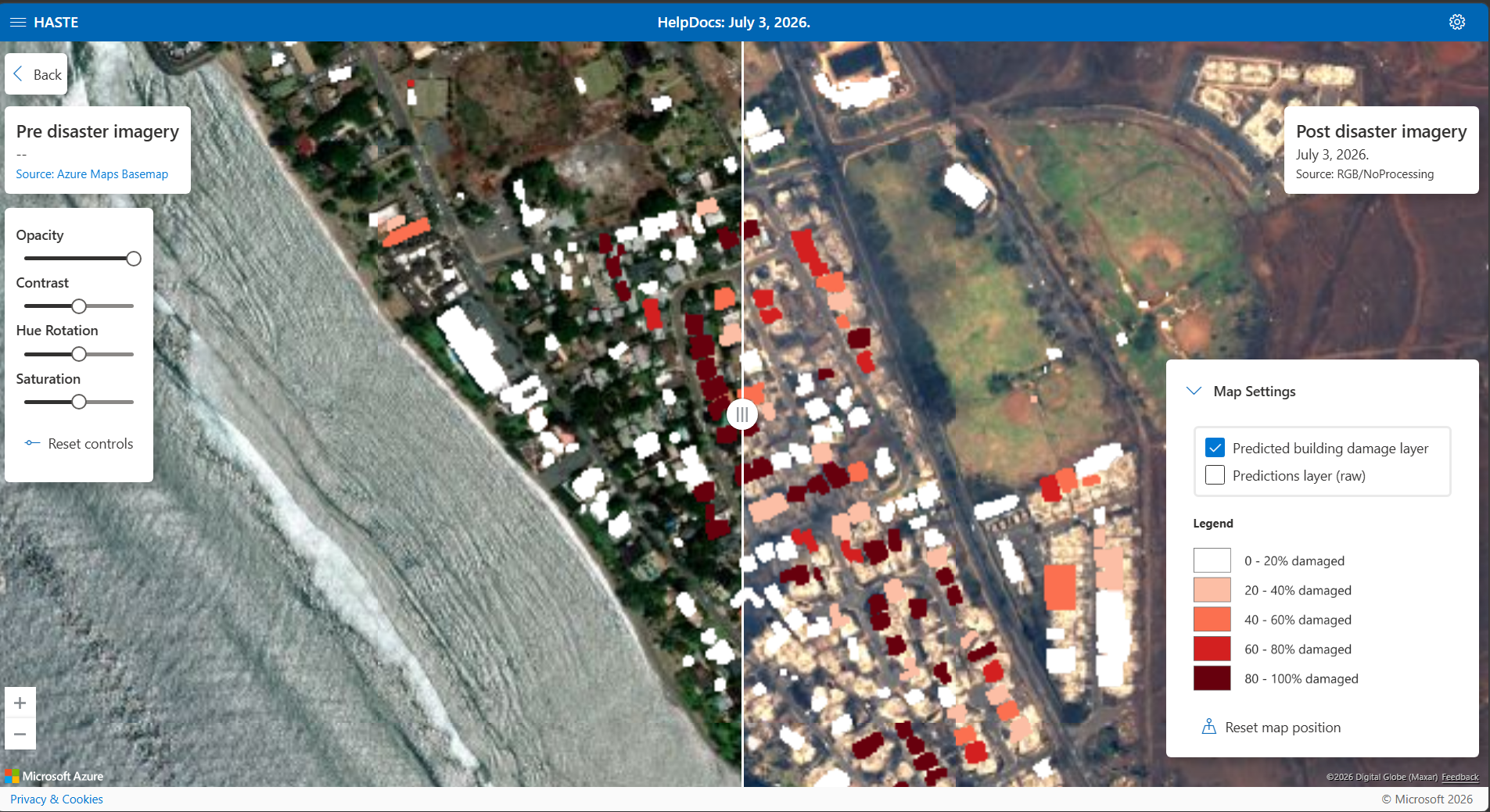
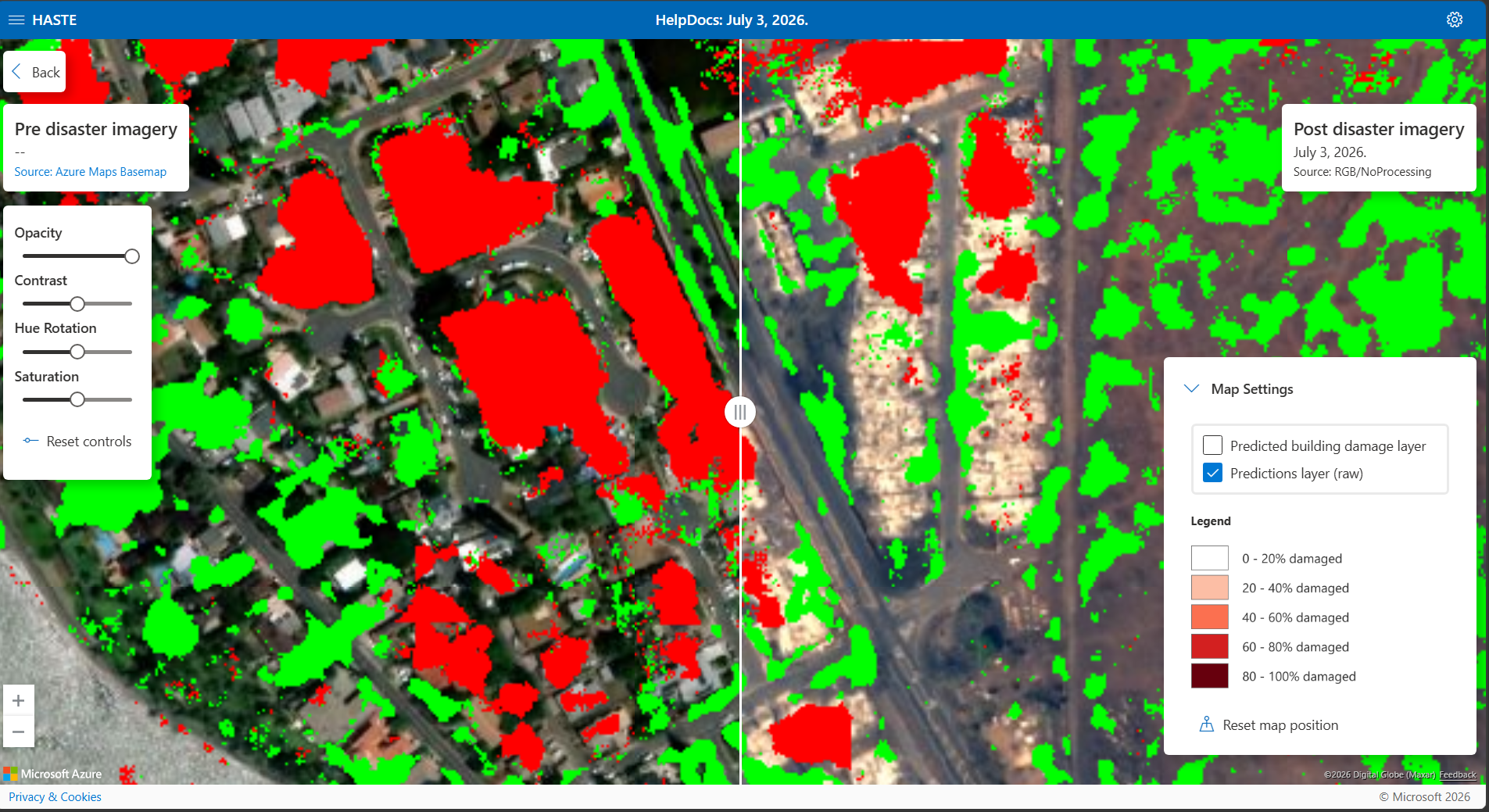
View opens the visualizer: the pre- and post-event imagery side by side with a swipe
control, the predicted damage layer overlaid on both, and an optional raw predictions
layer you can toggle on. Imagery sliders (opacity, contrast, hue, saturation) and keyboard
shortcuts — A (all pre-event), S (split), D (all post-event) — help you inspect and
share the result. See Keyboard shortcuts for the complete
reference.
Download the outputs#
Download Geopackage (
.gpkg) — the predicted damage layer.Download Training Artifacts — the training outputs (saved labels, checkpoints, logs).
Download Inference Artifacts — the inference outputs (predictions and building footprints).
Each download shows its file size.
Publish the dataset#
If your administrator has enabled publishing, the Results menu also offers Publish dataset… — archive the result as a downloadable copy or share it to a Planetary Computer STAC catalog. See Publishing datasets.
Reports#
If you’ve validated buildings for this layer, the Results menu also offers a Validation Report (accuracy, per-class precision/recall/F1, and a confusion matrix against your validation labels) and an Assessment Report (a damage summary and a damaged-building population estimate with a 95% confidence interval). These are the same reports described under Rapid Building Assessment.