Rapid Building Assessment#
Goal: go from imagery to a per-building damage map in minutes — no model training job required. HASTE computes a compact “fingerprint” (an embedding) for every building footprint, you label a handful of buildings, and a fast in-browser model predicts damage for all of them. You then validate a sample and get accuracy metrics plus a damaged-building estimate.
This is the recommended path when you have building footprints and want a quick answer. For a continuous, pixel-level damage raster instead, see Damage Mapping with a Trained Model.
The workflow at a glance
Building layer → Embed → Interactive Label (label a few, model predicts the rest) → Predict all buildings → Validate a sample → Reports.
Before you start#
Create a project and add an image layer with the Building workflow selected, then load your pre-/post-event imagery — building footprints are prepared automatically during preprocessing. See Projects and Image layers. A building-workflow layer shows an Embed button once its status is Processed.
Footprints are sourced automatically from Overture Maps, or you can supply your own — see Custom building footprints.
Try it with sample data
New to HASTE? Use the Black River sample from Image layers (see
Sample data to try HASTE): create a Building-workflow layer with
black-river_visual_mosaic_cog.tif as the post-event imagery and
black-river_footprints.gpkg as the custom footprints.
Step 1 — Embed the buildings#
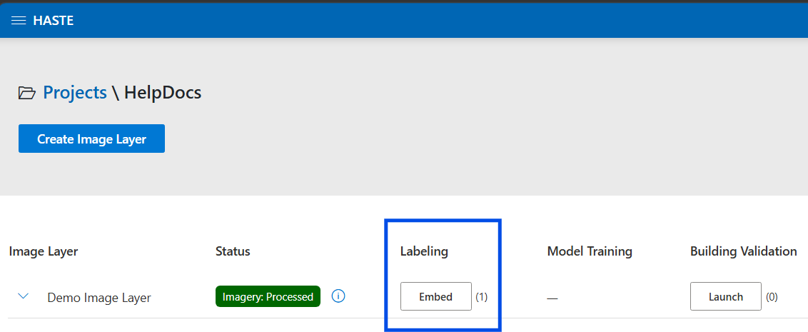
On the image layer, click the Embed button:
In the New Embedding dialog, configure:
Embedding backbone — MOSAIKS (random convolutional features) or DINOv2 (ViT-S/14 or ViT-B/14). MOSAIKS is the lightweight default.
Output dimensions — features per building (MOSAIKS only; default 1024).
Resize factor — how much to upscale the crop around each footprint (default 4 for MOSAIKS).
Batch size — how many buildings to process at once.
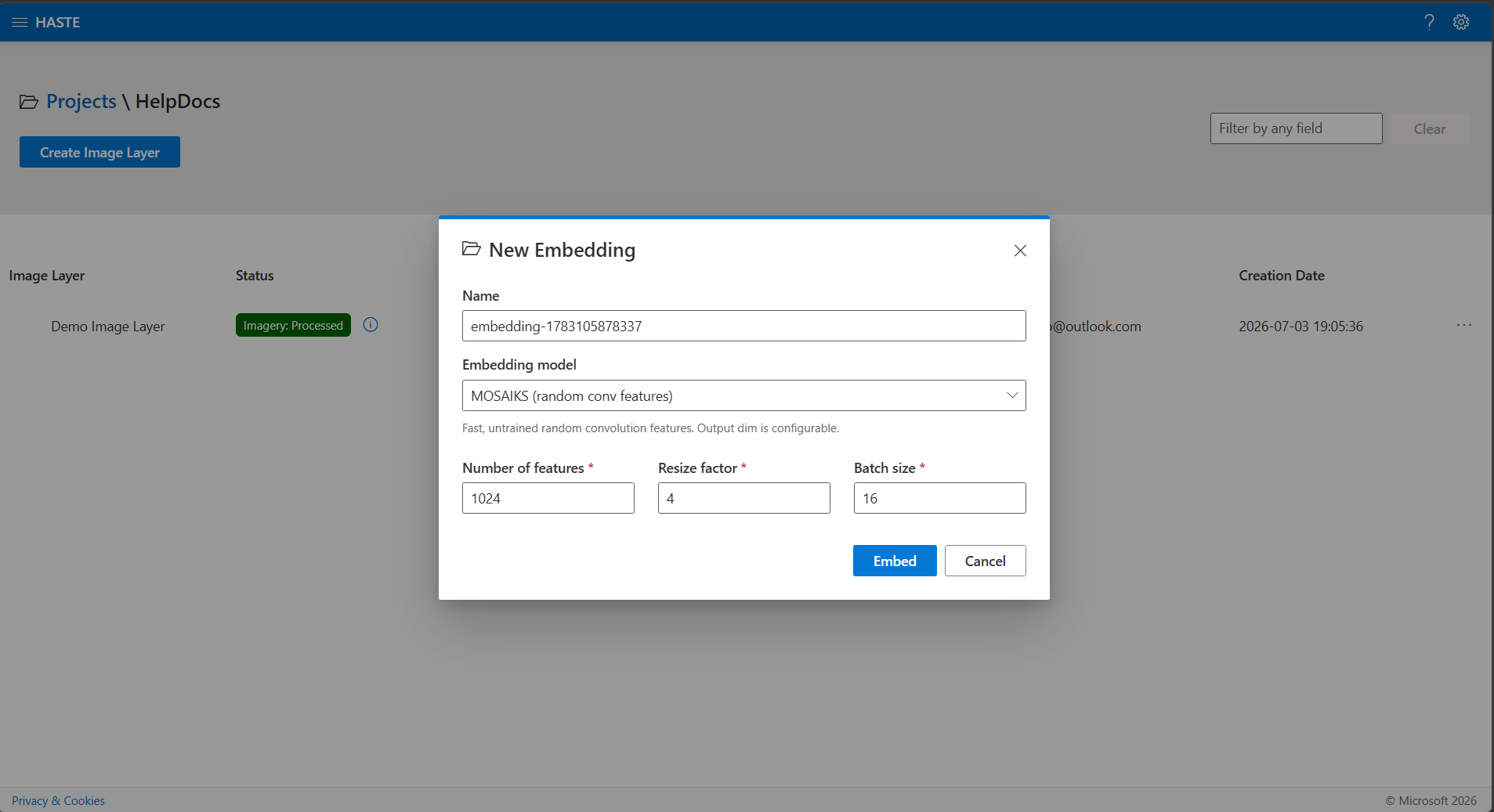
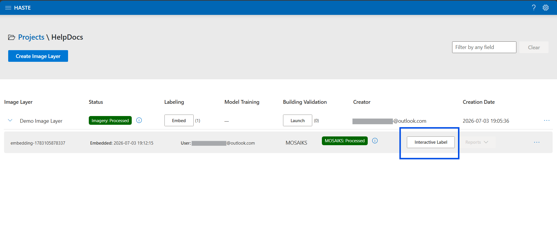
Click Embed to queue the job. It analyzes the imagery around every footprint, producing a feature vector per building plus vector tiles (PMTiles) for fast map display. When it finishes, an embedding row appears with an Interactive Label button.
Tip
An embedding is a compact set of numbers capturing what each building looks like in the imagery. Similar-looking buildings get similar embeddings — which is what lets a small model generalize your labels to every building.
Step 2 — Label interactively#
Click Interactive Label to open the map-based labeler: satellite imagery (with a pre-/post-event toggle), building footprints (visible at zoom 15 and closer), and a side panel with the class selector, counts, a view toggle, and quality metrics.
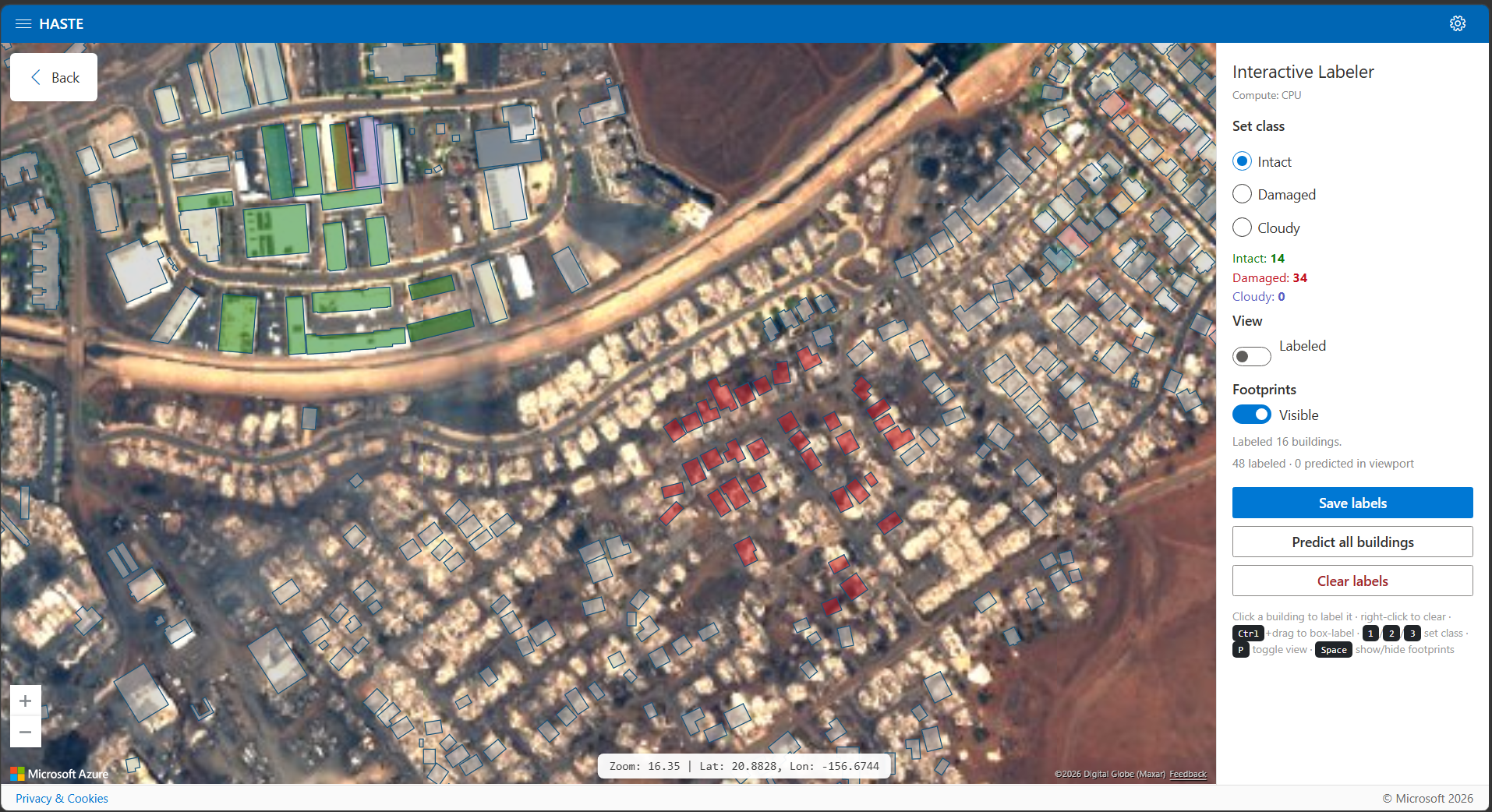
Left-click a building to label it with the selected class; right-click to remove a label.
Ctrl+drag (Cmd+drag on macOS) to box-select and label many buildings at once.
Classes: Intact (green), Damaged (red), Cloudy (purple) for obscured buildings; unlabeled buildings are gray.
Shortcuts:
1/2/3pick a class,Tcycles,Ptoggles Labeled/Predicted view,Spaceshows/hides footprints, andCtrl+dragbox-labels buildings. Swipe comparison is on by default;A/S/Dmove its divider left/to an even split/right. See Keyboard shortcuts for the complete reference.
Once you’ve labeled at least 3 buildings in each of 2+ classes, an in-browser model (logistic regression, WebGPU-accelerated when available) trains automatically and predicts damage for every building in view. Toggle View: Labeled ↔ Predicted to compare. The panel shows holdout precision / recall / F1 for the Damaged class so you can watch quality improve as you label diverse examples.
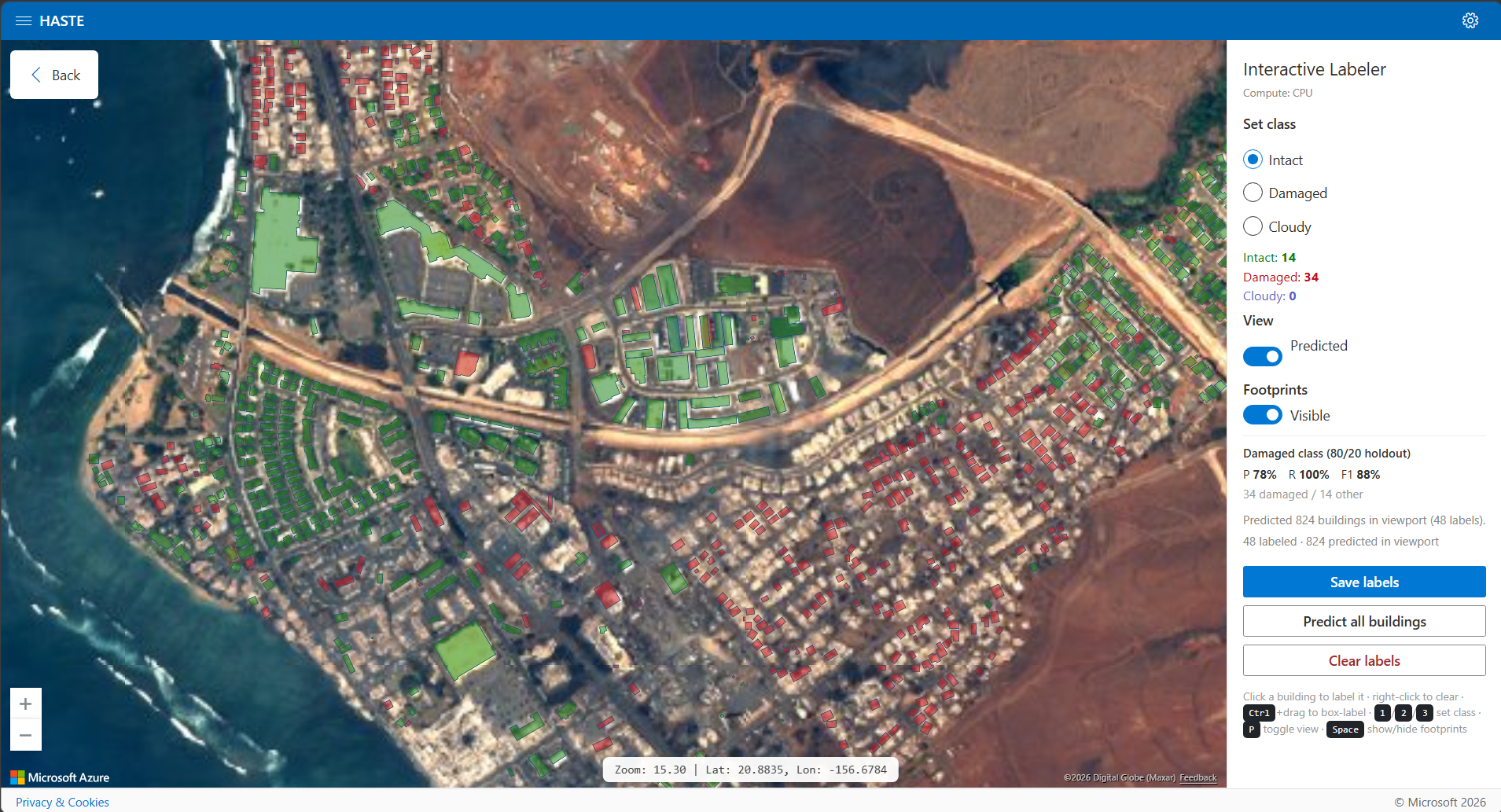
Under Advanced, Show misclassified buildings trains or reuses the current in-browser model and highlights only human-labeled buildings whose current prediction differs. Correctly classified and unlabeled buildings are not highlighted. This view is mutually exclusive with Predicted and Uncertainty views and turns off if labels fall below the training threshold.
Step 3 — Predict all buildings#
Save labels persists your manual labels so you can resume later (no full prediction).
Predict all buildings trains on all your labels, scores every building, and saves the result as a predictions layer (a GeoPackage) — this unlocks the reports below.
Clear labels removes your labels (including the saved copy); it cannot be undone.
Important
Labels and predictions are tied to a specific embedding. If footprints don’t respond to labeling or look stale, the layer likely needs to be re-embedded — re-run Embed and open the new embedding row.
Step 4 — Validate a sample#
Open Building Validation for the layer to spot-check the predictions. It loads a random sample of footprints (~200 by default) with the pre-/post-event imagery.
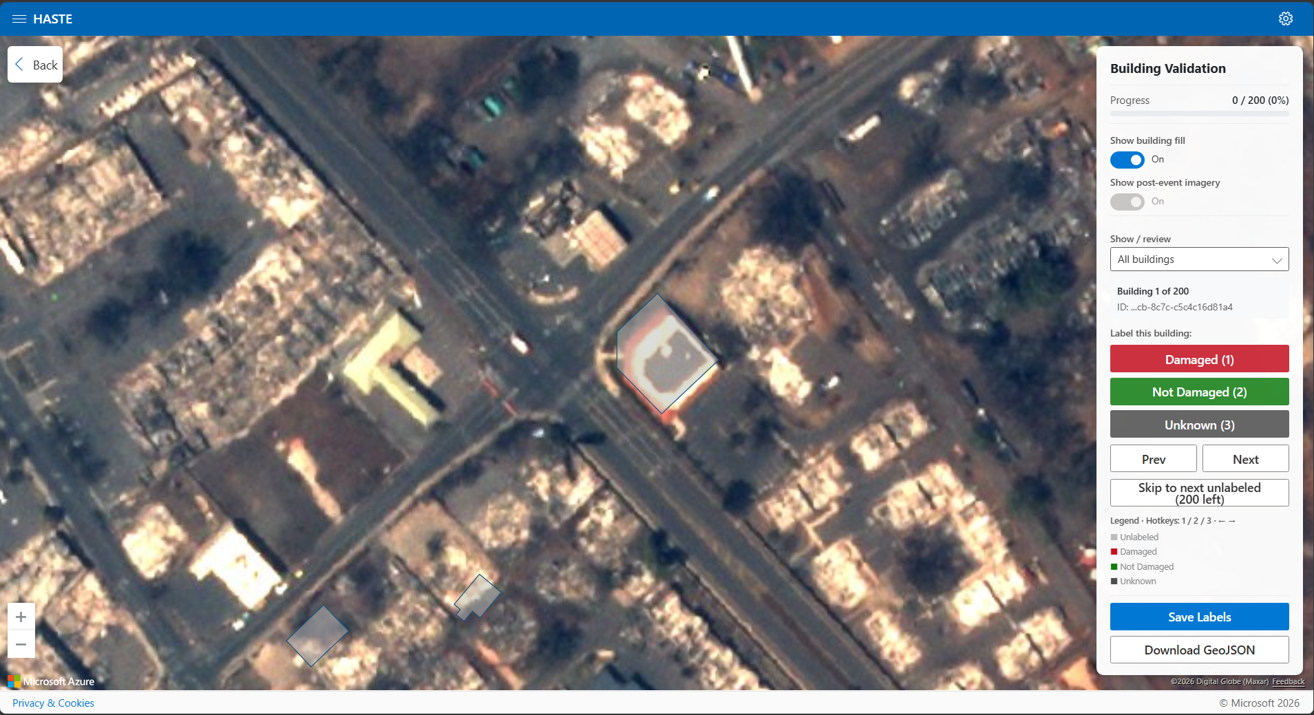
Select a building and label it Damaged, Not Damaged, or Unknown.
Shortcuts:
1/2/3to label; arrow keys to move Prev/Next (auto-advances to the next unlabeled);Ashows pre-event imagery (or basemap) andDshows post-event imagery. Filter by label status; a progress bar tracks your coverage.Save Labels to persist, or Download GeoJSON to export the labeled sample.
These human labels are the ground truth the reports compare predictions against (Unknown labels are excluded from metrics).
Step 5 — Review the reports#
From the embedding row’s Reports menu:
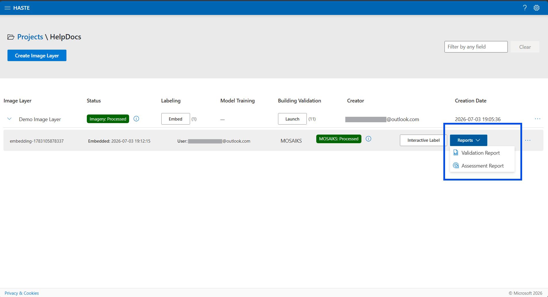
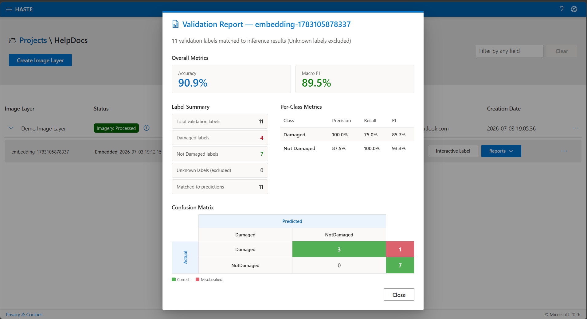
Validation Report — matches predictions against your validation labels: overall accuracy, per-class precision/recall/F1 (Damaged, Not Damaged), macro-F1, and a confusion matrix.
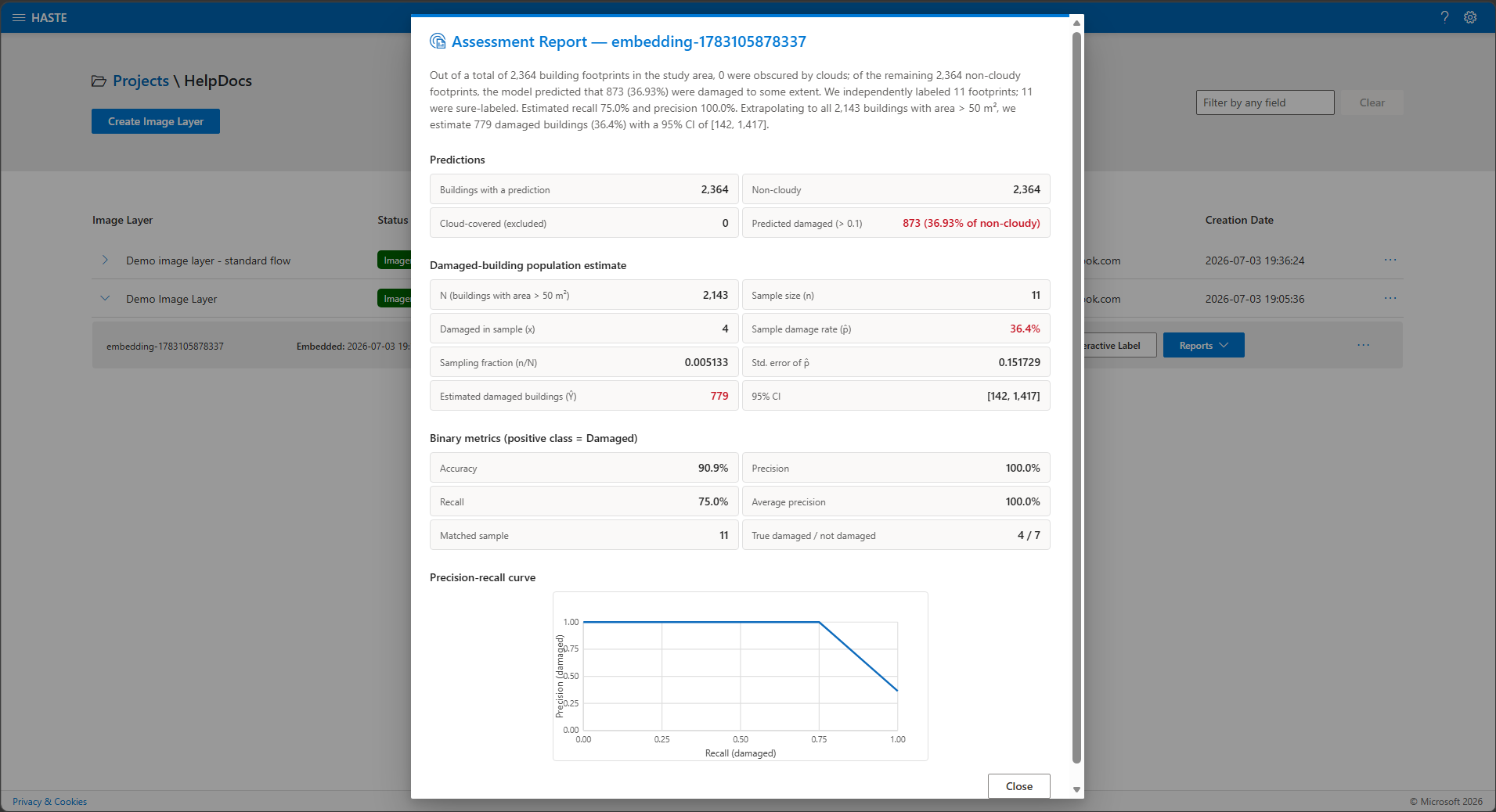
Assessment Report — summarizes predictions across the layer (total, scored vs. cloud-excluded, count and % predicted damaged) and, using your validation sample, estimates the total damaged buildings with a 95% confidence interval, plus a precision–recall curve.
Publish the dataset#
If your administrator has enabled publishing, you can also Publish dataset… from the embedding row — archive the assessment as a downloadable copy or share it to a Planetary Computer STAC catalog. See Publishing datasets.
Tips#
Label a diverse set of buildings (varied roofs, colors, damage severity) rather than many similar ones.
Use Cloudy for cloud-obscured buildings so they’re excluded from scoring.
Watch the Damaged-class F1; if recall is low, add more damaged examples before running Predict all buildings.