Demo: Using create_odds_ratios from the vivainsights Python Package
This notebook demonstrates how to use the create_odds_ratios function from the vivainsights Python package to analyze the relationship between ordinal metrics and an independent variable.
In this walkthrough, you will:
Load demo data (
pq_data) from the package.Create an independent variable (
UsageSegments_12w) usingidentify_usage_segments.Compute favorability scores for ordinal metrics with
compute_fav.Calculate odds ratios for ordinal metrics using
create_odds_ratios.Visualize the results for easier interpretation.
[1]:
# Import necessary libraries
import vivainsights as vi
import pandas as pd
import warnings

# Suppress warnings for cleaner output
warnings.filterwarnings("ignore")
Step 1: Load the demo data
First, load the sample Person Query dataset (pq_data) provided by vivainsights.
[2]:
# Load the demo data
pq_data = vi.load_pq_data()

# Display the first few rows of the dataset
pq_data.head()
[2]:
| PersonId | MetricDate | Collaboration_hours | Copilot_actions_taken_in_Teams | Meeting_and_call_hours | Internal_network_size | Email_hours | Channel_message_posts | Conflicting_meeting_hours | Large_and_long_meeting_hours | ... | Summarise_chat_actions_taken_using_Copilot_in_Teams | Summarise_email_thread_actions_taken_using_Copilot_in_Outlook | Summarise_meeting_actions_taken_using_Copilot_in_Teams | Summarise_presentation_actions_taken_using_Copilot_in_PowerPoint | Summarise_Word_document_actions_taken_using_Copilot_in_Word | FunctionType | SupervisorIndicator | Level | Organization | LevelDesignation | |
|---|---|---|---|---|---|---|---|---|---|---|---|---|---|---|---|---|---|---|---|---|---|
| 0 | bf361ad4-fc29-432f-95f3-837e689f4ac4 | 2024-03-31 | 17.452987 | 4 | 11.767599 | 92 | 7.523189 | 0.753451 | 2.079210 | 0.635489 | ... | 2 | 0 | 0 | 0 | 0 | Specialist | Manager | Level3 | IT | Senior IC |
| 1 | 0500f22c-2910-4154-b6e2-66864898d848 | 2024-03-31 | 32.860820 | 6 | 26.743370 | 193 | 11.578396 | 0.000000 | 8.106997 | 1.402567 | ... | 2 | 0 | 4 | 1 | 0 | Specialist | Manager | Level2 | Legal | Senior Manager |
| 2 | bb495ec9-8577-468a-8b48-e32677442f51 | 2024-03-31 | 21.502359 | 8 | 13.982031 | 113 | 9.073214 | 0.894786 | 3.001401 | 0.000192 | ... | 1 | 1 | 0 | 0 | 0 | Manager | Manager | Level4 | Legal | Junior IC |
| 3 | f6d58aaf-a2b2-42ab-868f-d7ac2e99788d | 2024-03-31 | 25.416502 | 4 | 16.895513 | 131 | 10.281204 | 0.528731 | 1.846423 | 1.441596 | ... | 0 | 0 | 0 | 0 | 0 | Manager | Manager | Level1 | HR | Executive |
| 4 | c81cb49a-aa27-4cfc-8211-4087b733a3c6 | 2024-03-31 | 11.433377 | 4 | 6.957468 | 75 | 5.510535 | 2.288934 | 0.474048 | 0.269996 | ... | 0 | 0 | 1 | 0 | 0 | Technician | Manager | Level1 | Finance | Executive |
5 rows × 73 columns
Step 2: Create the independent variable with identify_usage_segments
Use identify_usage_segments to classify users into usage segments based on their Copilot actions. The independent variable (UsageSegments_12w) is created by aggregating columns that start with Copilot_actions_taken_in_.
[3]:
# Identify usage segments
usage_segments_data = vi.identify_usage_segments(
    data=pq_data,
    metric_str=[
        "Copilot_actions_taken_in_Teams",
        "Copilot_actions_taken_in_Outlook",
        "Copilot_actions_taken_in_Excel",
        "Copilot_actions_taken_in_Word",
        "Copilot_actions_taken_in_Powerpoint"
    ],
    version="12w",
    return_type="data"
)

# Display the first few rows of the updated dataset
usage_segments_data.head()
[3]:
| PersonId | MetricDate | Collaboration_hours | Copilot_actions_taken_in_Teams | Meeting_and_call_hours | Internal_network_size | Email_hours | Channel_message_posts | Conflicting_meeting_hours | Large_and_long_meeting_hours | ... | Level | Organization | LevelDesignation | target_metric | target_metric_l12w | target_metric_l4w | IsHabit12w | IsHabit4w | UsageSegments_12w | UsageSegments_4w | |
|---|---|---|---|---|---|---|---|---|---|---|---|---|---|---|---|---|---|---|---|---|---|
| 0 | 01986072-719a-404c-ae98-009d92e82323 | 2024-03-31 | 26.884733 | 7 | 17.700027 | 156 | 9.667004 | 0.117751 | 2.674868 | 1.262361 | ... | Level4 | IT | Junior IC | 10 | 10.00 | 10.00 | False | False | Novice User | Novice User |
| 1 | 01986072-719a-404c-ae98-009d92e82323 | 2024-04-07 | 21.280727 | 10 | 15.372990 | 121 | 8.417014 | 0.519473 | 0.368913 | 2.108141 | ... | Level4 | IT | Junior IC | 12 | 11.00 | 11.00 | False | False | Novice User | Novice User |
| 2 | 01986072-719a-404c-ae98-009d92e82323 | 2024-04-14 | 17.450330 | 8 | 11.808617 | 104 | 7.889519 | 1.907069 | 0.096829 | 0.853150 | ... | Level4 | IT | Junior IC | 11 | 11.00 | 11.00 | False | False | Novice User | Novice User |
| 3 | 01986072-719a-404c-ae98-009d92e82323 | 2024-04-21 | 21.368059 | 3 | 14.908550 | 115 | 6.776404 | 0.209775 | 3.953832 | 0.878616 | ... | Level4 | IT | Junior IC | 4 | 9.25 | 9.25 | False | True | Novice User | Habitual User |
| 4 | 01986072-719a-404c-ae98-009d92e82323 | 2024-04-28 | 20.849744 | 5 | 13.737000 | 110 | 8.759793 | 0.931585 | 1.201305 | 0.000000 | ... | Level4 | IT | Junior IC | 6 | 8.60 | 8.25 | False | True | Novice User | Habitual User |
5 rows × 80 columns
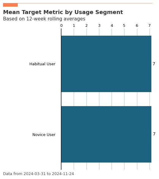
Visualize the mean of target_metric by usage segment
To better understand usage behavior, create a bar plot showing the mean of target_metric grouped by UsageSegments_12w.
[4]:
# Visualize the mean of `target_metric` by `UsageSegments_12w`
usage_segments_bar_plot = vi.create_bar(
    data=usage_segments_data,
    metric="target_metric",
    hrvar="UsageSegments_12w",
    return_type="plot",
    plot_title="Mean Target Metric by Usage Segment",
    plot_subtitle="Based on 12-week rolling averages"
)

# Display the bar plot
usage_segments_bar_plot.show()
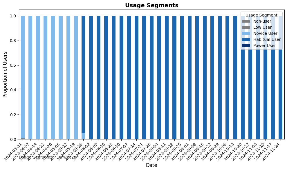
Visualize usage segments over time
Next, visualize the distribution of usage segments over time using identify_usage_segments with return_type='plot'. The following shows a horizontal stacked bar plot, which shows the evolution in the proportion of the usage segments over time.
[8]:
# Visualize usage segments over time
usage_segments_time_plot = vi.identify_usage_segments(
    data=pq_data,
    metric_str=[
        "Copilot_actions_taken_in_Teams",
        "Copilot_actions_taken_in_Outlook",
        "Copilot_actions_taken_in_Excel",
        "Copilot_actions_taken_in_Word",
        "Copilot_actions_taken_in_Powerpoint"
    ],
    version="12w",
    return_type="plot"
)

# Display the time plot
usage_segments_time_plot.show()
Step 3: Compute favorability scores for ordinal metrics
Before calculating odds ratios, use compute_fav() to convert ordinal metrics into categorical variables representing favorable and unfavorable scores. This standardizes metrics to a 100-point scale, making results easier to interpret and compare.
Neutral scores are dropped to focus on the most meaningful responses.
In usage_segments_data printed below, it can be seen that compute_fav() has added several columns suffixing the ordinal_metrics columns with _100 and _fav.
[9]:
# Define the ordinal metrics
ordinal_metrics = [
    "eSat",
    "Initiative",
    "Manager_Recommend",
    "Resources",
    "Speak_My_Mind",
    "Wellbeing",
    "Work_Life_Balance",
    "Workload"
]

# Compute favorability scores
usage_segments_data = vi.compute_fav(
    data=usage_segments_data,
    ord_metrics=ordinal_metrics,
    item_options=5,  # Assuming a 5-point scale for ordinal metrics
    fav_threshold=70,
    unfav_threshold=40,
    drop_neutral=True
)

# Display the first few rows of the updated dataset
usage_segments_data.head()
[9]:
| PersonId | MetricDate | Collaboration_hours | Copilot_actions_taken_in_Teams | Meeting_and_call_hours | Internal_network_size | Email_hours | Channel_message_posts | Conflicting_meeting_hours | Large_and_long_meeting_hours | ... | Resources_100 | Resources_fav | Speak_My_Mind_100 | Speak_My_Mind_fav | Wellbeing_100 | Wellbeing_fav | Work_Life_Balance_100 | Work_Life_Balance_fav | Workload_100 | Workload_fav | |
|---|---|---|---|---|---|---|---|---|---|---|---|---|---|---|---|---|---|---|---|---|---|
| 36 | 02723512-4f45-4385-8d1a-c23048e1e961 | 2024-04-07 | 26.310260 | 1 | 17.635230 | 124 | 10.887553 | 0.000000 | 3.322255 | 0.067661 | ... | 25.0 | unfav | 25.0 | unfav | 100.0 | fav | 0.0 | unfav | 0.0 | unfav |
| 83 | 02c55079-f137-4abb-9806-f58e9b60efd6 | 2024-06-30 | 17.401642 | 4 | 10.399207 | 84 | 5.253439 | 0.195852 | 3.203440 | 0.975272 | ... | 25.0 | unfav | 25.0 | unfav | 100.0 | fav | 0.0 | unfav | 0.0 | unfav |
| 123 | 02ddc980-8f37-4156-9397-6d621e445a00 | 2024-08-04 | 20.612899 | 3 | 14.130869 | 103 | 8.070390 | 0.577123 | 1.374351 | 0.000000 | ... | 25.0 | unfav | 25.0 | unfav | 100.0 | fav | 0.0 | unfav | 0.0 | unfav |
| 135 | 02ddc980-8f37-4156-9397-6d621e445a00 | 2024-10-27 | 19.514361 | 2 | 10.986860 | 91 | 6.221707 | 2.286118 | 2.294472 | 0.391576 | ... | 25.0 | unfav | 25.0 | unfav | 100.0 | fav | 0.0 | unfav | 0.0 | unfav |
| 164 | 032432ad-390c-4ce4-9f25-d5be080bd982 | 2024-09-15 | 34.160594 | 3 | 27.364673 | 182 | 12.926987 | 0.197464 | 6.306590 | 1.153810 | ... | 25.0 | unfav | 25.0 | unfav | 100.0 | fav | 0.0 | unfav | 0.0 | unfav |
5 rows × 96 columns
Step 4: Calculate odds ratios for ordinal metrics
Now, calculate odds ratios for the favorability scores of these ordinal metrics:
eSatInitiativeManager_RecommendResourcesSpeak_My_MindWellbeingWork_Life_BalanceWorkload
The independent variable is UsageSegments_12w.
[13]:
# Calculate odds ratios
odds_ratios_table = vi.create_odds_ratios(
    data=usage_segments_data,
    ord_metrics=ordinal_metrics,
    metric="UsageSegments_12w",
    return_type="table"
)

# Display the odds ratios table
print(odds_ratios_table)
   UsageSegments_12w Level  Odds_Ratio     Ordinal_Metric      n
0      Habitual User     1    1.000000               eSat    3.0
1        Novice User     1    1.000000               eSat    1.0
2      Habitual User     2   53.571429               eSat  135.0
3        Novice User     2   37.000000               eSat   49.0
4      Habitual User     4   18.142857               eSat   58.0
5        Novice User     4   10.333333               eSat   14.0
6      Habitual User     5    0.428571               eSat    1.0
7        Novice User     5    0.333333               eSat    NaN
8      Habitual User     1    1.000000         Initiative    4.0
9        Novice User     1    1.000000         Initiative    3.0
10     Habitual User     2   54.333333         Initiative  166.0
11       Novice User     2   18.142857         Initiative   57.0
12     Habitual User     4    1.444444         Initiative    6.0
13       Novice User     4    1.571429         Initiative    5.0
14     Habitual User     1    1.000000  Manager_Recommend    5.0
15       Novice User     1    1.000000  Manager_Recommend    NaN
16     Habitual User     2   43.545455  Manager_Recommend  163.0
17       Novice User     2  133.000000  Manager_Recommend   59.0
18     Habitual User     4    1.909091  Manager_Recommend   10.0
19       Novice User     4    7.000000  Manager_Recommend    3.0
20     Habitual User     5    0.090909  Manager_Recommend    NaN
21       Novice User     5    5.000000  Manager_Recommend    2.0
22     Habitual User     1    1.000000          Resources    2.0
23       Novice User     1    1.000000          Resources    NaN
24     Habitual User     2  100.600000          Resources  171.0
25       Novice User     2  141.000000          Resources   62.0
26     Habitual User     4    0.600000          Resources    1.0
27       Novice User     4    3.000000          Resources    1.0
28     Habitual User     1    1.000000      Speak_My_Mind    2.0
29       Novice User     1    1.000000      Speak_My_Mind    1.0
30     Habitual User     2   97.400000      Speak_My_Mind  166.0
31       Novice User     2   43.666667      Speak_My_Mind   58.0
32     Habitual User     4    3.800000      Speak_My_Mind    9.0
33       Novice User     4    3.666667      Speak_My_Mind    5.0
34     Habitual User     4    1.000000          Wellbeing   74.0
35       Novice User     4    1.000000          Wellbeing   24.0
36     Habitual User     5    1.786885          Wellbeing  123.0
37       Novice User     5    1.938776          Wellbeing   43.0
38     Habitual User     1    1.000000  Work_Life_Balance  143.0
39       Novice User     1    1.000000  Work_Life_Balance   49.0
40     Habitual User     2    0.352785  Work_Life_Balance   58.0
41       Novice User     2    0.321101  Work_Life_Balance   17.0
42     Habitual User     1    1.000000           Workload  143.0
43       Novice User     1    1.000000           Workload   51.0
44     Habitual User     2    0.317829           Workload   54.0
45       Novice User     2    0.252174           Workload   14.0
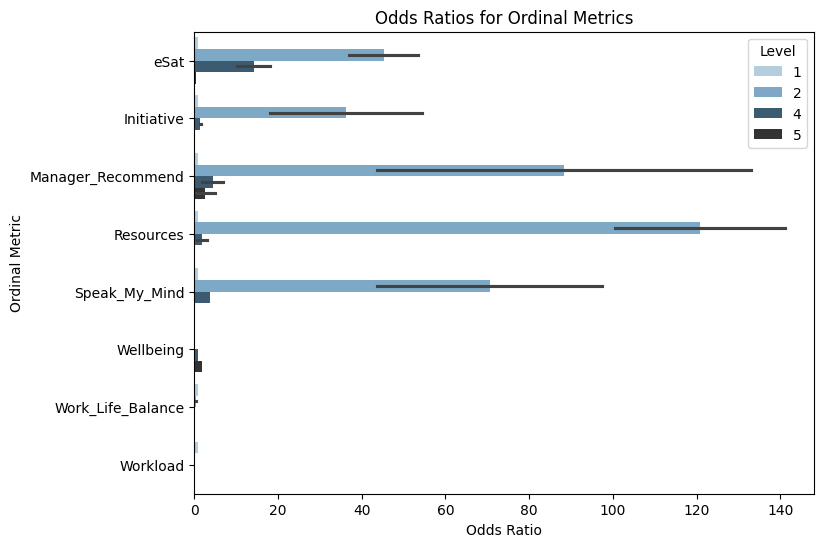
Since favorability columns with the values fav, unfav, and neu have already been created using compute_fav(), you can use these directly in the proportional odds model to simplify the analysis.
When interpreting odds ratios, a value greater than 1 indicates that the odds of a favorable outcome are higher for the group compared to the reference group, while a value less than 1 means the odds are lower. An odds ratio of exactly 1 suggests no difference between groups. This helps you understand how different usage segments are associated with the likelihood of favorable responses on each metric.
[14]:
# Define ordinal metrics with '_fav' suffix
ordinal_metrics_fav = [f"{metric}_fav" for metric in ordinal_metrics]

# Calculate odds ratios
odds_ratios_table_fav = vi.create_odds_ratios(
    data=usage_segments_data,
    ord_metrics=ordinal_metrics_fav,
    metric="UsageSegments_12w",
    return_type="table"
)

# Display the odds ratios table
print(odds_ratios_table_fav)
   UsageSegments_12w  Level  Odds_Ratio         Ordinal_Metric    n
0      Habitual User    fav    1.000000               eSat_fav   59
1        Novice User    fav    1.000000               eSat_fav   14
2      Habitual User  unfav    2.953488               eSat_fav  137
3        Novice User  unfav    3.645161               eSat_fav   50
4      Habitual User    fav    1.000000         Initiative_fav    6
5        Novice User    fav    1.000000         Initiative_fav    5
6      Habitual User  unfav   38.230769         Initiative_fav  168
7        Novice User  unfav   12.090909         Initiative_fav   59
8      Habitual User    fav    1.000000  Manager_Recommend_fav   10
9        Novice User    fav    1.000000  Manager_Recommend_fav    5
10     Habitual User  unfav   23.285714  Manager_Recommend_fav  167
11       Novice User  unfav   12.090909  Manager_Recommend_fav   59
12     Habitual User    fav    1.000000          Resources_fav    1
13       Novice User    fav    1.000000          Resources_fav    1
14     Habitual User  unfav  169.000000          Resources_fav  172
15       Novice User  unfav   47.000000          Resources_fav   62
16     Habitual User    fav    1.000000      Speak_My_Mind_fav    9
17       Novice User    fav    1.000000      Speak_My_Mind_fav    5
18     Habitual User  unfav   25.842105      Speak_My_Mind_fav  167
19       Novice User  unfav   12.090909      Speak_My_Mind_fav   59
20     Habitual User    fav    1.000000          Wellbeing_fav  172
21       Novice User    fav    1.000000          Wellbeing_fav   63
22     Habitual User  unfav    1.000000  Work_Life_Balance_fav  172
23       Novice User  unfav    1.000000  Work_Life_Balance_fav   63
24     Habitual User  unfav    1.000000           Workload_fav  172
25       Novice User  unfav    1.000000           Workload_fav   63
[ ]:
# Filter for Level == 'fav' only, and sort Odds_Ratio in descending order
odds_ratios_table_fav = odds_ratios_table_fav[odds_ratios_table_fav['Level'] == 'fav']
odds_ratios_table_fav = odds_ratios_table_fav.sort_values(by='Odds_Ratio', ascending=False)

print(odds_ratios_table_fav)
   UsageSegments_12w Level  Odds_Ratio         Ordinal_Metric    n
4      Habitual User   fav         1.0         Initiative_fav    6
5        Novice User   fav         1.0         Initiative_fav    5
8      Habitual User   fav         1.0  Manager_Recommend_fav   10
16     Habitual User   fav         1.0      Speak_My_Mind_fav    9
9        Novice User   fav         1.0  Manager_Recommend_fav    5
12     Habitual User   fav         1.0          Resources_fav    1
1        Novice User   fav         1.0               eSat_fav   14
17       Novice User   fav         1.0      Speak_My_Mind_fav    5
13       Novice User   fav         1.0          Resources_fav    1
21       Novice User   fav         1.0          Wellbeing_fav   63
0      Habitual User   fav         1.0               eSat_fav   59
20     Habitual User   fav         1.0          Wellbeing_fav  172
Step 5: Visualize the odds ratios
Create a bar plot to visualize the odds ratios for the ordinal metrics, making it easier to compare the impact of usage segments.
[20]:
# Visualize odds ratios
odds_ratios_plot = vi.create_odds_ratios(
    data=usage_segments_data,
    ord_metrics=ordinal_metrics,
    metric="UsageSegments_12w",
    return_type="plot"
)

# Display the plot
odds_ratios_plot.show()
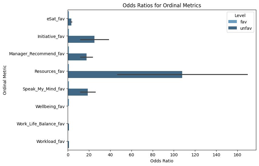
[22]:
# Visualize odds ratios for favorability
odds_ratios_plot_fav = vi.create_odds_ratios(
    data=usage_segments_data,
    ord_metrics=ordinal_metrics_fav,
    metric="UsageSegments_12w",
    return_type="plot"
)

# Display the plot
odds_ratios_plot_fav.show()
Summary
In this notebook, you learned how to:
Load demo data (
pq_data).Create an independent variable (
UsageSegments_12w) usingidentify_usage_segments.Compute favorability scores for ordinal metrics with
compute_fav.Calculate odds ratios for ordinal metrics using
create_odds_ratios.Visualize the results for interpretation.
By combining create_odds_ratios with compute_fav, you can consistently analyze the relationship between ordinal metrics and independent variables, regardless of the original point scale.