Brief Overview
What is Bioininformatics
“Bioinformatics is an interdisciplinary field that develops methods and software tools for understanding biological data.”” 1
History
Bioinformatics or Computational Biology was born in the 1960s. 2 This was due to 3 items:
- Expanding collection of amino acid sequences
- Increase need for computational power to answer these questions and study protein biology
- Access to academic computers was not longer a major problem
At its basics, bioinformatics is the convergence of computational methods, data, mathematics and biology to answer questions in biological sciences. 2
Why is Bioininformatics important
New measurement techniques produce huge amounts of biological data. We need advanced data analytical methods, and increasing computational resources, to fully understand the data. Typically data sources are scattered and produce noisy data with missing values.
Technologies and data formats
DNA sequencing technologies
Overview of the Sanger method, first sequencing method:
- sequencing by synthesis (not degradation)
- primers hybridize to DNA
- polymerase + dNTPS + ddNTP terminators at low concentration
- 1 lane per base, visually interpret ladder
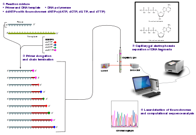
(Image curtesy of Wikipedia)
Timeline of DNA Sequencing technologies:
- 2005: 454 (Roche)
- 2006: Solexa (Illumina)
- 2007: ABI/SOLiD (Life Technologies)
- 2010: Complete Genomics
- 2011: Pacific Biosciences
- 2010: Ion Torrent (Life Technologies)
- 2015: Oxford Nanopore Technologies
Key terms of the future of Sequencing:
- Massively parallel” sequencing
- “High-throughput” sequencing
- “Ultra high-throughput” sequencing
- “Next generation” sequencing (NGS)
- “Second generation” sequencing
Data Formats
- Many different types of data
- Standard formats exists for many of them
Below is a list of common file formats
Comprehensive list of formats available at UCSC Genome Browser.
Tables
Standard format for keeping tables of data, metadata.
| field1 | field2 | field3 | |:——:|:——:|:——–:| | - | - | - |
Fields (colimns) seperated by a chacter on each line:
- Comma (or Character) Separated Vector (CSV)
- Tab Separated Vector (TSV)
- Some have column name as first row (header), some don’t
FASTA
A sequence in FASTA format begins with a single-line description, followed by lines of sequence data. The definition line (defline) is distinguished from the sequence data by a greater-than (>) symbol at the beginning. The word following the “>” symbol is the identifier of the sequence, and the rest of the line is the description (optional).
SampleSequence QIKDLLVSSSTDLDTTLVLVNAIYFKGMWKTAFNAEDTREMPFHVTKQESKPVQMMCMNNSFNVATLPAE KMKILELPFASGDLSMLVLLPDEVSDLERIEKTINFEKLTEWTNPNTMEKRRVKVYLPQMKIEEKYNLTS
FASTQ
Each read/pair has a unique name. A read has the sequence and the quality of each nucleotide sequence.
@read_name sequences_nucleotides +read_name quality_of_each_nucelotdie_in_ASCII
SAM/BAM/CRAM
- Alignments are kept in SAM format
- SAM is sorted and compressed into BAM or CRAM
- One line per alignment
header
The header starts with @
- @HD: header definition
- @SQ: a sequence in the reference file you used followd by how long it was and it’s comment (from the reference file)
- @RG: read groups you assinged while mapping the reads
- @PG: programs used to obtain this alignemnt, in order
body
- Each line keeps an alignment
- Each aligned has 11 mandatory fields
| Col | Field | Type | Brief description |
|---|---|---|---|
| 1 | QNAME | String | Query template NAME |
| 2 | FLAG | Int | bitwise FLAG |
| 3 | RNAME | String | References sequence NAME |
| 4 | POS | Int | 1- based leftmost mapping POSition |
| 5 | MAPQ | Int | MAPping Quality |
| 6 | CIGAR | String | CIGAR string |
| 7 | RNEXT | String | Ref. name of the mate/next read |
| 8 | PNEXT | Int | Position of the mate/next read |
| 9 | TLEN | Int | observed Template LENgth |
| 10 | SEQ | String | segment SEQuence |
| 11 | QUAL | String | ASCII of Phred-scaled base QUALity+33 |
@HD VN:1.6 SO:coordinate @SQ SN:ref LN:47 ref 516 ref 1 0 14M2D31M * 0 0 AGCATGTTAGATAAGATAGCTGTGCTAGTAGGCAGTCAGCGCCAT * r001 99 ref 7 30 14M1D3M = 39 41 TTAGATAAAGGATACTG *
- 768 ref 8 30 1M * 0 0 * * CT:Z:.;Warning;Note=Ref wrong? r002 0 ref 9 30 3S6M1D5M * 0 0 AAAAGATAAGGATA * PT:Z:1;4;+;homopolymer r003 0 ref 9 30 5H6M * 0 0 AGCTAA * NM:i:1 r004 0 ref 18 30 6M14N5M * 0 0 ATAGCTTCAGC * r003 2064 ref 31 30 6H5M * 0 0 TAGGC * NM:i:0 r001 147 ref 39 30 9M = 7 -41 CAGCGGCAT * NM:i:1
(Example curtesy of Samtools)
VCF
- Variant Call Format
- Stored in Tab seperated format
header
- Manadtory header lines: information about the fields (columns) starting with ##INFO
- Extra: filtering, metadata, tools, …
body
- Fixed Fields
- CHROM - chromosome
- POS - position
- ID - identifier
- REF - reference base(s): Each base must be one of A,C,G,T,N (case insensitive).
- ALT - alternate base(s): Comma separated list of alternate non-reference alleles.
- QUAL - quality: Phred-scaled quality score for the assertion made in ALT.
- FILTER - filter status
- INFO - additional information
##fileformat=VCFv4.2 ##fileDate=20090805 ##source=myImputationProgramV3.1 ##reference=file:///seq/references/1000GenomesPilot-NCBI36.fasta ##contig=<ID=20,length=62435964,assembly=B36,md5=f126cdf8a6e0c7f379d618ff66beb2da,species=”Homo sapiens”,taxonomy=x> ##phasing=partial ##INFO=<ID=NS,Number=1,Type=Integer,Description=”Number of Samples With Data”> ##INFO=<ID=DP,Number=1,Type=Integer,Description=”Total Depth”> ##INFO=<ID=AF,Number=A,Type=Float,Description=”Allele Frequency”> ##INFO=<ID=AA,Number=1,Type=String,Description=”Ancestral Allele”> ##INFO=<ID=DB,Number=0,Type=Flag,Description=”dbSNP membership, build 129”> ##INFO=<ID=H2,Number=0,Type=Flag,Description=”HapMap2 membership”> ##FILTER=<ID=q10,Description=”Quality below 10”> ##FILTER=<ID=s50,Description=”Less than 50% of samples have data”> ##FORMAT=<ID=GT,Number=1,Type=String,Description=”Genotype”> ##FORMAT=<ID=GQ,Number=1,Type=Integer,Description=”Genotype Quality”> ##FORMAT=<ID=DP,Number=1,Type=Integer,Description=”Read Depth”> ##FORMAT=<ID=HQ,Number=2,Type=Integer,Description=”Haplotype Quality”> #CHROM POS ID REF ALT QUAL FILTER INFO FORMAT NA00001 NA00002 NA00003 20 14370 rs6054257 G A 29 PASS NS=3;DP=14;AF=0.5;DB;H2 GT:GQ:DP:HQ 0|0:48:1:51,51 1|0:48:8:51,51 1/1:43:5:.,. 20 17330 . T A 3 q10 NS=3;DP=11;AF=0.017 GT:GQ:DP:HQ 0|0:49:3:58,50 0|1:3:5:65,3 0/0:41:3 20 1110696 rs6040355 A G,T 67 PASS NS=2;DP=10;AF=0.333,0.667;AA=T;DB GT:GQ:DP:HQ 1|2:21:6:23,27 2|1:2:0:18,2 2/2:35:4 20 1230237 . T . 47 PASS NS=3;DP=13;AA=T GT:GQ:DP:HQ 0|0:54:7:56,60 0|0:48:4:51,51 0/0:61:2 20 1234567 microsat1 GTC G,GTCT 50 PASS NS=3;DP=9;AA=G GT:GQ:DP 0/1:35:4 0/2:17:2 1/1:40:3
Genomic regions (BED/GFF/GTF)
- A region is defined by three required fields
- sequence name
- start coordinate
- end coordinate
- Define regions of interest introls, exons, genes, etc.
- No headers
- Addtional information saved as fields after the first three
- Many formats extend common tab-seperated formats: BED, GFF, GTF UCSC Genome Browser.
BED
Mandatory fields:
- chrom - Name of the chromosome/sequence reference
- chromStart - 0-based starting position of the feature
- chromEnd - Ending position of the feature
chr1 11182 1200 chr3 3 2000 chrX 4000 50001
GFF
- seqname - The name of the sequence. Must be a chromosome or scaffold.
- source - The program that generated this feature.
- feature - The name of this type of feature. Some examples of standard feature types are “CDS” “start_codon” “stop_codon” and “exon”li>
- start - The starting position of the feature in the sequence. The first base is numbered 1.
- end - The ending position of the feature (inclusive).
- score - A score between 0 and 1000. If the track line useScore attribute is set to 1 for this annotation data set, the score value will determine the level of gray in which this 7. feature is displayed (higher numbers = darker gray). If there is no score value, enter “.”.
- strand - Valid entries include “+”, “-“, or “.” (for don’t know/don’t care).
- frame - If the feature is a coding exon, frame should be a number between 0-2 that represents the reading frame of the first base. If the feature is not a coding exon, the value should be “.”.
- group - All lines with the same group are linked together into a single item.
chr22 TeleGene enhancer 10000000 10001000 500 + . touch1 chr22 TeleGene promoter 10010000 10010100 900 + . touch1 chr22 TeleGene promoter 10020000 10025000 800 - . touch2
GTF
- Extenssion of GFF2, backward compatible
- First eight GTF fields are the same as GFF
- feature fields is the same as GFF, has controlled vocabullary:
- gene, transcript, exon, CDS, 5UTR, 3UTR, inter, inter_CSN, etc
- group field expanded into a list of attributes (i.e. key/value pairs)
- attribute list must begin with the two mandatory attributes:
- gene_id value - A globally unique identifier for the genomic source of the sequence.
- transcript_id value - A globally unique identifier for the predicted transcript.
Example of the ninth field in a GTF data line:
gene_id “Em:U62317.C22.6.mRNA”; transcript_id “Em:U62317.C22.6.mRNA”; exon_number 1
Genomic Analysis Basics
The process of making genomic data ready for analysis can be broken down into a couple of distinct stages.
- Sequencing/Primary Analysis
- Secondary Analysis
- Tertiary Analysis
Sequencing/Primary Analysis
At this stage, scientist extract DNA/RNA from a source such as tissue or saliva. Once the DNA is extracted, it’s then prepared and sequenced. There are a couple of assays available today based on the particular question:
- DNA binding
- ChIP-seq
- DNA accesibility
- ATAC-seq
- DNase-seq
- DNA methylation
- Whole Genome Bisulfite Sequencing
- Reduced Represntation Bisulfite Sequencing
- DNA Sequencing
- Whole Exome Sequencing
- Whole Genome Sequencing
- 3D chromatin Structure
- Hi-C
- Transcription
- bulk RNA-seq
- microRNA-seq
- single-cell RNA-seq
We will focus on Whole Genome Sequencing (WGS) in this overview.
Prepare
Due to limitations with current sequencing technology, the first stage of processing requires the DNA molecule to be fragmented into smaller segments. These segments called short reads are about 100-200 base pairs long. To increase the confidence in the output, hundreds of copies of this short reads are duplicated. This redundancy as we’ll see later is by design to increase output confidence.
Sequence
These short reads are then processed by the sequencing equipment which uses fluorescence technology to read each base at a time. This process called base calling, results in a file based output called a base call library. Most sequencers include a post processing step that will convert this raw output to a user friendly format, and accounting for the base call quality. The more commonly used file formats include FASTQ or BAM. This will be the starting point of most of the analysis that we’ll perform. Sequencing technology is not perfect, errors in base calling are not uncommon.
Secondary Analysis
The next step in the process is to take these short reads and reassemble them to a representation of the original genome. As you can imagine this is a fairly complex and computationally intensive process. This is made possible because the Human Genome Project produced a version of the human genome that’s commonly accepted as the reference genome. FYI, this genome is not the genome of a single person but instead it’s a composite genome of a group of people.
Think of this reference genome as the cover picture of a million piece jigsaw puzzle and the short reads as the individual pieces. The first step is to use computer algorithms to figure out where each short read fits in the original genome. As discussed earlier, there’s usually more than one copy for each short read. As the alignment process continues to process the reads, the more short reads that cover a given area of the genome, the more confidence that the short reads are accurate and that they are accurately aligned. You will hear scientist and analyst talk of coverage with a given number say 50X. The higher the number, the more confidence in the sequence/alignment process. The more sensitive the use, the higher the coverage is expected.
There are different alignment tools out there, but the one that we’ll use is called the Borrows-Wheeler-Aligner(BWA). The final output of the aligment is a alignment map, usually represented as a BAM file(.bam).
The last step in the secondary analysis is variant calling. Now that we have a representation of the sequenced genome, we compare that against the reference genome and find any areas where our genome of study varies from the reference genome. These areas are called variants and are the focus of subsequent analysis.
One thing to note, the presence of a variant does not indicate a problem, it’s an area of interest. Most variants are benign (not disease causing), while some are pathogenic (disease causing). When performing downstream analysis, researchers can compare the variants against already identified and annotated variants.
There are many types of variants. Variants are usually classified based on the the number of bases involved. The smallest variant is a single base variant, commonly known as a Single Nucleotide Variant(SNV). This type of variant is usually a change in the letter code of the DNA, for example where the reference genome might have a T, our genome of study might have a C. If a SNV is present in more than 1% of the population, it’s referred to as a Single Nucleotide Polymorphism(SNP).
Other common types of variants are Insertions and Deletions, also commonly referred to as InDels. These could be an insertion of a small number of bases or large number of bases.
The largest types of variants would be changes to the entire chromosome, these are called Whole Chromosome Aneuploidy. In some rare changes during cell division/multiplation (Mitosis & Meisosis), problems can result in either a loss of a chromosome (monosomy), or a gain of a chromosome(Trisomy). This a usually survivable but with corresponding health complications. For example, Trisomy of Chromosome 21 results in an extra 21st chromosome which causes Downs Syndrome. In very rare cases, the process of mitosis/meiosis can result in a gain of a new chromosome for all 23 chromosomes, a condition called Triploidy or a loss of a single chromosome for all 23 chromosomes, a condition called Monoploidy. This are usually fatal and the cell doesn’t survive.
Tertiary Analysis
Tertiary analysis is finally the step that we start to ask questions of the genomic data that we’ve acquired. One of the questions we’ll try to answer here is whether any of the variants that we found in the previous section are associated with a particular disease.
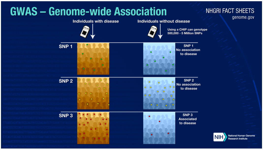
One of the tools used to accomplish this is called a Genome Wide Association Study(GWAS). So what’s a GWAS and how is it conducted?
In a GWAS researchers will find two groups of people, one group that is known to have a particular attribute (could be a disease or any other physical attribute), and a control group that doesn’t have the attribute. Both groups will have their DNA sequenced. The variants will then be analyzed, GWAS usually focus on SNPs.
Let’s assume that the particular attribute of interest is caused by a particular SNP. You’d expect to see these SNPs in higher frequency in the affected group and in lower frequency in the control group. In the image below, you can see how concentration of SNP 3 in the affected group is higher than in the control group. Therefore you can conclude that SNP 3 is associated with the attribute of interest.
GWAS have been used successfully to identify genetic variations that contribute to risk for various diseases. For example, three independent studies 3 found that age-related macular degeneration (which leads to blindness) is associated with variation in the gene (Complement Factor H) which produces a protein involved in regulating inflammation.
Other diseases that have been studied and shown to be associated with genetic variation include:
- Diabetes
- Parkison’s disease
- Some heart disorders
- Obesity
- Crohn’s disease
- Response to anti-depressant medications
Current challenges
The research community is facing a data challenge. The cost of sequencing has been following rapidly, coupled with additionally high-throughput technologies, more data will be generated than ever before. Additionally, these data sources aren’t generated in isolation, but rather are thought about together coupled and should be integrated with a growing clinical data. Below outlines some of the challenges facing researchers today and where a shift to the Cloud can help.
Infrastructure
The community has to consider purchasing, supporting and maintaining the following ():
- Scalable computing
- Storage
- Network infrastructure
The cloud has offered solutions to the above issues by offering rapid availability and scalability. There are 4 types of infrastructures to consider:
- Public: the infrastructure exists on cloud provider premises and is managed by the cloud provider.
- Private: the infrastructure is provisioned and managed by exclusive use by a single organization.
- Community: collaborative effort where infrastructure exclusive used by a community of users.
- Hybrid: a composition of two or more distinct cloud infrastructures and are bound together to allow for portability and sharing.
Reproducibility
As compute resources have different configuration, ranging from hardware specifications to required software, the ability to run the same analysis across different infrastructures has become none trivial.
Three main challenges exist 4:
- Managing software versions and dependencies
- Managing computational environments
- Managing workflows (Languages and Engines)
- Languages
Provenance
Sufficient information should be tracked to capture all the requirements supporting reusability and reproducibility of the analysis.
Should store:
- Software versions
- Software parameters
- Data sources and produced during the workflows
FAIR Principles
Management of data must now commonly adhere to the FAIR principles 5:
- Findable: Metadata and data should be easy to find for both humans and computers.
- Accessible: Need to know how data can be accessed, including any authentication and authorization.
- Interoperable: Data needs to interoperate with applications, analysis, storage and processing.
- Reusable: Data should be well-described so they can be replicated and/or combined.
Security/Privacy
- Secure methods for transferring, storing and sharing data.
- Protect privacy of personal data in accordance with local privacy and data protection laws and requirements.