XGBoost Model Overview
The XGBoost Model for the Solution Template will do the following:
- Source and run step 1 to retrieve training and testing data
- Transform and use training data created in step 1 to train the xgboost model
- Use the trained model to perform prediction using testing data
- Save predicted results
- Evaluate model performance
- Output results (AUC, TPR, TNR)
The XGBoost Model for the Solution Template can be found in the script loanchargeoff_xgboost.R. The function to run the script is xgboost_model(). It can take in optional input parameters which specify the HDFS working and data directories, the local working directory, and the loan data. The input parameters are as follows:
Input Parameters for xgboost_model(): HDFSWorkDir, HDFSDataDir, LocalWorkDir, Loan_Data
Once the script has completed running on the data, the function outputs the model AUC, TPR, and TNR in the form of a list.
XGBoost Model Script Details
The process to incorporate the XGBoost model into the Solution Template was split into 3 primary steps including (1) Training, (2) Predicting, and (3) Scoring the model. Figure 1 below shows the flow of logic of the XGBoost model script for the Solution Template.
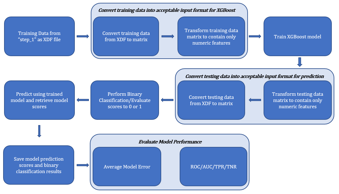
STEP 1: Training the Model
Input Format
The open-source XGBoost model in R takes in several types of input data including:
- Dense Matrix i.e. matrix
- Sparse Matrix i.e. Matrix::dgCMatrix
- Local Data Files e
- xgb.DMatrix
Data Conversion and Processing
In order to use the XGBoost model, the input data must be one of the four types above. When the step 1 of the Solution Template is applied, it creates training and testing data of the class RxXdfData (i.e. XDF files). Since XGBoost does not support XDF files as input, we must manipulate the data so that we can use the XGBoost model. The RevoScaleR function rxDataStep() was used to convert the data to an acceptable format for XGBoost. This rxDataStep()function is able to take an RxXdfData data source object as input and return a data.frame as output. When using this function to convert data types, it was necessary to explicitly set the parameter maxRowsByCols in the function to NULL. This prevents data from being truncated when the input dataset is over 3 million entries.
The open-source XGBoost model also requires input data to be completely numerical. Since the training dataset contains both numerical and categorical features, the data.matrix() function was then used to set all categorical data to NA and convert the data frame to a matrix. The resulting data was then of type matrix with only numerical data and was an acceptable input for the XGBoost model.
One final transformation involved removing the columns memberId, loanId, loan_open_date, and paydate from the training data as they represent ID numbers and dates which would not help improve model performance. The charge_off column was also removed because this is the label – or the data we want to predict – and as such should not be included in the training dataset. After this step, the transformed data was inputted to the XGBoost model for training.
Training the Model and Output Format
In order to train the XGBoost model, the xgboost() function was used with the following parameters:
- data = transformed training data
- label = charge off
- nrounds = 4
- max.depth = 4
- eta = 1
- nthread = 4
- objective = “binary:logistic” [The objective function “binary:logistic” is explained further in the Binary Classification section below.]
The output format for the trained XGBoost model is type list of class xgb.Booster.
STEP 2: Predicting Results
Data Conversion and Processing
In order to predict results, the testing data must be a matrix consistent with the training data. Therefore, rxDataStep() was also used on the testing data to convert it from an XDF file to a data frame. The categorical features were then set to NA using the function data.matrix(), and the charge_off column was removed from the data. The final result was a matrix of only numerical features and no charge_off column.
Prediction
To predict results, the predict() function was used with parameters including the trained model and the transformed testing data. The output from the prediction are probabilistic decimal scores between 0 and 1.
Binary Classification
Binary classification was used to ensure that all results are either a 0 or 1, to be consistent with the loan charge off results. The XGBoost model usually outputs score values which are decimals greater than 0. However, when the model is trained setting the objective function as binary:logistic, it scales these values to probabilistic decimal outputs between 0 and 1.
Therefore, our predicted scores after calling the predict() function are these probabilistic values between 0 and 1. Once we have these predicted scores, we can use the following simple formula to perform binary classification: if the result is greater than 0.5, classify the result as a 1, and if the result is less than or equal to 0.5, classify the result as a 0.
After applying this formula to our predicted scores, we obtain our final predicted results for loan charge off.
Saving Results
The testing data, predicted model scores, binary classification results, and observed results are saved as a single XDF file in the Hadoop Distributed File System.
STEP 3: Evaluation of Model Performance
Model Error
One metric used for model evaluation was calculating the error of the model as the mean of the instances when the predicted results did not equal the actual charge off results in the testing data. This measure is included as an additional useful metric within the script but is not an output of the function. This method yielded about a 0.85% model error.
NOTE : For purposes of this documentation, the data used was Loan_Data100000.csv. All scores reflect usage of this dataset
True Positive Rate (TPR) and True Negative Rate (TNR)
The True Positive Rate (TPR) was another metric used for model evaluation. The TPR, also known as Sensitivity, is the ratio of positives that are correctly identified to the total number of positives identified. The TPR score of the predicted results for the XGBoost model was 0.9734.
The True Negative Rate (TNR) was another metric used for model evaluation. The TNR, also known as Specificity, is the ratio of negatives that are correctly identified to the total number of negatives identified. The TNR score of the predicted results for the XGBoost model was 0.9912.
ROC Curve and AUC
The ROC, or Receiver Operating Characteristic, curve is commonly used with binary classifiers as a way to picture the tradeoff between sensitivity and specificity of the model. The ROC curve plots the False Positive Rate (1-TNR) on the x-axis against the True Positive Rate on the y-axis. Since the graph is inversely proportional to the number of actual negatives in the x-direction and actual positives in the y-direction, the graph always starts at coordinate x=0, y=0 and ends at coordinate x=1, y=1. The ideal location to be on the ROC curve would be at x=0,y=1 as this point represents a False Positive Rate of 0 and a True Positive Rate of 1 (i.e. the case when we categorize all positives correctly). For this to happen, the ROC curve should ideally bend as close to the point x=0, y=1 as possible so the area under the ROC curve would also be as close to 1 as possible. Therefore, the Area Under the Curve (AUC) is a good single value metric of how ideal the ROC curve is; when the AUC is closer to 1, it generally implies a better ROC curve and model performance. The AUC of the XGBoost model was calculated to be 0.9988.