For the Data Scientist - Develop with R
- Step 0: Create Intermediate Directories
- Step 1: Merging and Cleaning
- Step 2: Splitting and Feature Engineering
- Step 3: Training, Testing and Evaluating
- Step 4: Operational Metrics Computation and Scores Transformation
Loan Credit Risk
When a financial institution examines a request for a loan, it is crucial to assess the risk of default to determine whether to grant it. This solution is based on simulated data for a small personal loan financial institution, containing the borrower’s financial history as well as information about the requested loan. View more information about the data.
Scores is created in SQL Server. This data is then visualized in PowerBI.
To try this out yourself, visit the Quick Start page.
Below is a description of what happens in each of the steps: data preparation, feature engineering, model development, prediction, and deployment in more detail.
Development Stage
The Modeling or Development stage includes five steps:
- Step 0: Create intermediate directories
- Step 1: Data processing
- Step 2: Splitting and Feature engineering
- Step 3: Training, testing and evaluation
- Step 4: Operational metrics computation and scores transformation
They will all be invoked by the development_main.R script for this development stage. This script also:
- Opens the Spark connection.
- Lets the user specify the paths to the working directories on the edge node and HDFS. We assume they already exist.
- Lets the user specify the paths to the data sets Loan and Borrower on HDFS. (The data is synthetically generated by sourcing the data_generation.R script.)
- Creates a directory, LocalModelsDir, that will store the model and other tables for use in the Production or Web Scoring stages (inside the loan_dev main function).
- Updates the tables of the Production stage directory, ProdModelDir, with the contents of LocalModelsDir (inside the loan_dev main function).
Step 0: Intermediate Directories Creation
In this step, we create or clean intermediate directories both on the edge node and HDFS. These directories will hold all the intermediate processed data sets in subfolders.
Related files:
- step0_directories_creation.R
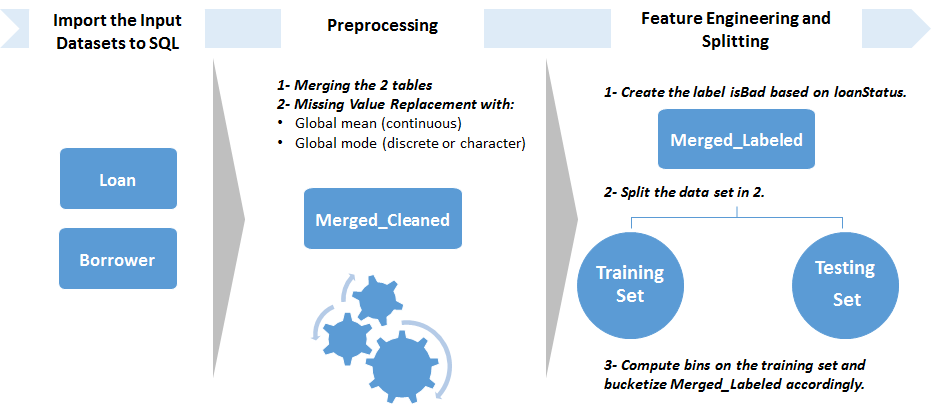
Step 1: Merging and Cleaning
In this step, the raw data is loaded into SQL in two tables called Loan and Borrower. They are then merged into one, Merged.
Then, if there are missing values, the data is cleaned by replacing missing values with the mode (categorical variables) or mean (float variables). This assumes that the ID variables (loanId and memberId) as well as loanStatus do not contain blanks.
The cleaned data is written to the SQL table Merged_Cleaned. The Statistics are written to SQL if you want to run a batch scoring from SQL after a development stage in R.
Input:
- Raw data: Loan.csv and Borrower.csv.
Output:
LoanandBorrowerSQL tables with the raw data.Merged_CleanedSQL table , with missing values replaced if applicable.StatsSQL table , with global means or modes for every variable.
In order to speed up the computations in this step and the following ones, we first convert the input data to .xdf files stored in HDFS. We convert characters to factors at the same time. We then merge the xdf files with the rxMerge function, which writes the xdf result to the HDFS directory “Merged”.
Finally, we want to fill the missing values in the merged table. Missing values of numeric variables will be filled with the global mean, while character variables will be filled with the global mode.
This is done in the following way:
- Use rxSummary function on the HDFS directory holding the merged table xdf files. This will give us the names of the variables with missing values, their types, the global means, as well as counts table through which we can compute the global modes.
- Save these statistics information to be used for the Production or Web Scoring stages, in the directory LocalModelsDir.
- If no missing values are found, the merged data splits are copied to the folder “MergedCleaned” on HDFS, without missing value treatment.
If there are missing values, we:
- Compute the global means and modes for the variables with missing values by using the rxSummary results.
- Define the “Mean_Mode_Replace” function which will deal with the missing values. It will be called in rxDataStep function which acts on the xdf files of “Merged”.
- Apply the rxDataStep function.
We end up with the cleaned splits of the merged table, “MergedCleaned” on HDFS.
Input:
- Working directories on the edge node and HDFS.
- 2 Data Tables: Loan and Borrower (paths to csv files)
Output:
- The statistics summary information saved to the local edge node in the LocalModelsDir folder.
- Cleaned raw data set MergedCleaned on HDFS in xdf format.
Related files:
- step1_preprocessing.R
Step 2: Splitting and Feature Engineering
For feature engineering, we want to design new features:
- Categorical versions of all the numeric variables. This is done for interpretability and is a standard practice in the Credit Score industry.
isBad: the label, specifying whether the loan has been charged off or has defaulted (isBad= 1) or if it is in good standing (isBad= 0), based onloanStatus.
This is done by following these steps:
-
Create the label
isBadwithrxDataStepfunction into the tableMerged_Labeled.Create the label isBad with rxDataStep function. Outputs are written to the HDFS directory “MergedLabeled”. We create at the same time the variable hashCode with values corresponding to hashing loanId to integers. It will be used for splitting. This hashing function ensures repeatability of the splitting procedure.
-
Split the data set into a training and a testing set. This is done by selecting randomly 70% of
loanIdto be part of the training set. In order to ensure repeatability,loanIdvalues are mapped to integers through a hash function, with the mapping andloanIdwritten to theHash_IdSQL table. The splitting is performed prior to feature engineering instead of in the training step because the feature engineering creates bins based on conditional inference trees that should be built only on the training set. If the bins were computed with the whole data set, the evaluation step would be rigged.Split the data set into a training and a testing set. This is done by selecting randomly a proportion (equal to the user-specified splitting ratio) of the MergedLabeled data. The output is written to the “Train” directory.
-
Compute the bins that will be used to create the categorical variables with
smbinning. Because some of the numeric variables have too few unique values, or because the binning function did not return significant splits, we decided to manually specify default bins in case smbinning does not return the splits. These default bins have been determined through an analysis of the data or through runningsmbinningon a larger data set. Those cutoffs are saved in the directory LocalModelsDir, to be used for the Production or Web Scoring stages.The bins computation is optimized by running
smbinningin parallel across the different cores of the server, through the use ofrxExecfunction applied in a Local Parallel (localpar) compute context. TherxElemArgargument it takes is used to specify the list of variables (here the numeric variables names) we want to apply smbinning on. They are saved to SQL in case you want to run a production stage with SQL after running a development stage in R. - Bucketize the variables based on the computed/specified bins with the function
bucketize, wrapped into anrxDataStepfunction. The final output is written into the SQL tableMerged_Features.The final output is written into the HDFS directory MergedFeatures, in xdf format.Finally, we convert the newly created variables from character to factors, and save the variable information in the directory LocalModelsDir, to be used for the Production or Web Scoring stages. The data with the correct variable types is written to the directory “MergedFeaturesFactors” on HDFS.
Input:
(assume the cleaned data, MergedCleaned is already created there by Step 1)
Merged_CleanedSQL table.- Working directories on the edge node and HDFS.
- The splitting ratio, corresponding to the proportion of the input data set that will go to the training set.
Output:
Merged_FeaturesSQL table containing new features.Hash_IdSQL table containing theloanIdand the mapping through the hash function.BinsSQL table containing the serialized list of cutoffs to be used in a future Production stage.- Cutoffs saved to the local edge node in the LocalModelsDir folder.
- Factor information saved to the local edge node in the LocalModelsDir folder.
- Analytical data set with correct variable types
MergedFeaturesFactorson HDFS in xdf format.
Related files:
- step2_feature_engineering.R
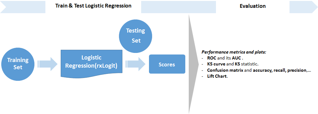
Step 3: Training, Testing and Evaluating
After converting the strings to factors (with stringsAsFactors = TRUE), we get the variables information (types and levels) of the Merged_Features SQL table with rxCreateColInfo. We then point to the training and testing sets with the correct column information.
In this step, we perform the following:
Split the xdf files in MergedFeaturesFactors into a training set, “Train”, and a testing set “Test”. This is done through rxDataStep functions, according to the splitting ratio defined and used in Step 2 and using the same hashCode created in Step 2.
Train a Logistic Regression on Train, and save it on the local edge node in the LocalModelsDir folder. It will be used in the Production or Web Scoring stages.
Then we build a Logistic Regression Model on the training set. The trained model is serialized and uploaded to a SQL table Model if needed later, through an Odbc connection.
Training a Logistic Regression for loan credit risk prediction is a standard practice in the Credit Score industry. Contrary to more complex models such as random forests or neural networks, it is easily understandable through the simple formula generated during the training. Also, the presence of bucketed numeric variables helps understand the impact of each category and variable on the probability of default. The variables used and their respective coefficients, sorted by order of magnitude, are stored in the data frame Logistic_Coeff returned by the step 3 function.
Finally, we compute predictions on the testing set, as well as performance metrics:
- KS (Kolmogorov-Smirnov) statistic. The KS statistic is a standard performance metric in the credit score industry. It represents how well the model can differenciate between the Good Credit applicants and the Bad Credit applicants in the testing set. We also draw the KS plot which corresponds to two cumulative distributions of the predicted probabilities. One is a subset of the predictions for which the observed values were bad loans (is_bad = 1) and the other concerns good loans (is_bad = 0). KS will be the biggest distance between those two curves.
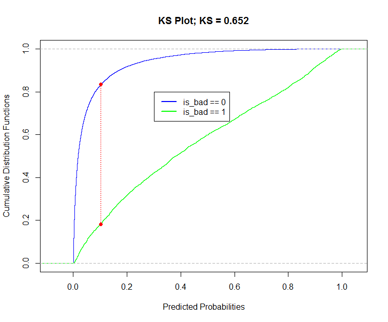
- Various classification performance metrics computed on the confusion matrix. These are dependent on the threshold chosen to decide whether to classify a predicted probability as good or bad. Here, we use as a threshold the point of the x axis in the KS plot where the curves are the farthest possible.
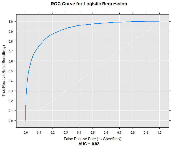
- AUC (Area Under the Curve) for the ROC. This represents how well the model can differenciate between the Good Credit applicants from the Bad Credit applicants given a good decision threshold in the testing set. We draw the ROC, representing the true positive rate in function of the false positive rate for various possible cutoffs.
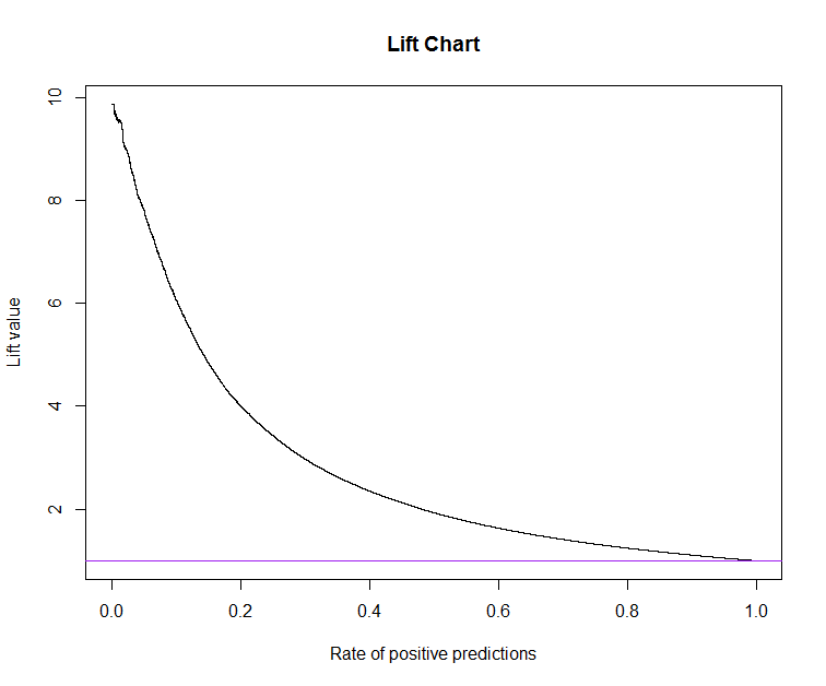
- The Lift Chart. The lift chart represents how well the model can perform compared to a naive approach. For instance, at the level where a naive effort could produce a 10% rate of positive predictions, we draw a vertical line on x = 0.10 and read the lift value where the vertical line crosses the lift curve. If the lift value is 3, it means that the model would produce 3 times the 10%, ie. 30% rate of positive predictions.
Input:
(assume the analytical data set, “MergedFeaturesFactors”, is already created there by Step 2)
Merged_FeaturesSQL table containing new features.Hash_IdSQL table containing theloanIdand the mapping through the hash function.- Working directories on the edge node and HDFS.
- The splitting ratio, corresponding to the proportion of the input data set that will go to the training set. It should be the same as the one used in Step 2.
Output:
ModelSQL table containing the serialized logistic regression model.Logistics_Coeffdata frame returned by the function. It contains variables names and coefficients of the logistic regression formula. They are sorted in decreasing order of the absolute value of the coefficients.Predictions_LogisticSQL table containing the predictions made on the testing set.Column_InfoSQL table containing the serialized list of factor levels to be used in a future Production stage.- Performance metrics returned by the step 3 function.
- Logistic Regression model saved to the local edge node in the LocalModelsDir folder.
- Logistic Regression formula saved to the local edge node in the LocalModelsDir folder.
- Prediction results given by the model on the testing set, “PredictionsLogistic” on HDFS in xdf format.
Related files:
- step3_train_score_evaluate.R
Step 4: Operational Metrics Computation and Scores Transformation
In this step, we create two functions compute_operational_metrics, and apply_score_transformation.
The first, compute_operational_metrics will:
-
Apply a sigmoid function to the output scores of the logistic regression, in order to spread them in [0,1] and make them more interpretable. This sigmoid uses the average predicted score, which is saved to SQL in case you want to run a production stage through SQL after a development stage with R.
-
Compute bins for the scores, based on quantiles (we compute the 1%-99% percentiles).
-
Take each lower bound of each bin as a decision threshold for default loan classification, and compute the rate of bad loans among loans with a score higher than the threshold.
It outputs the data frame Operational_Metrics,
which is also saved to SQL.
which is saved to the local edge node in the LocalModelsDir folder, for use in the Production and Web Scoring stages.
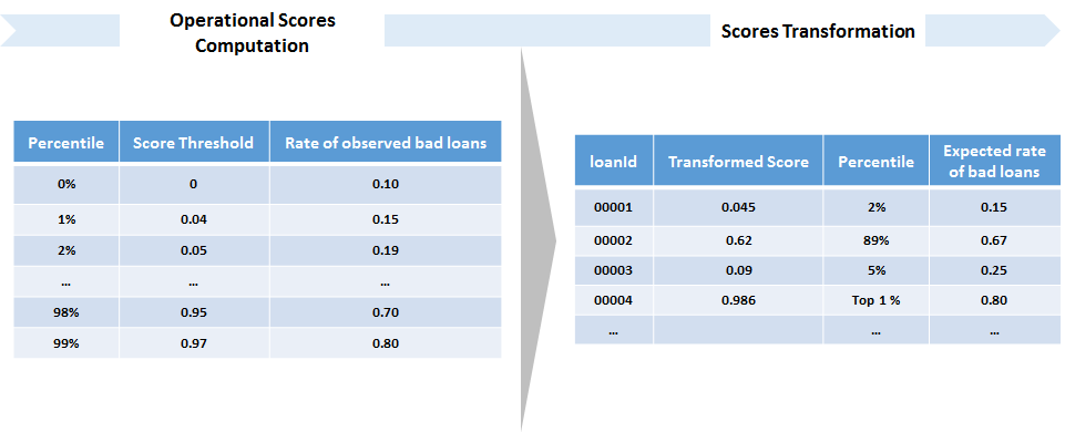
It can be read in the following way:
If the score cutoff of the 91th score percentile is 0.9834, and we read a bad rate of 0.6449, this means that if 0.9834 is used as a threshold to classify loans as bad, we would have a bad rate of 64.49%. This bad rate is equal to the number of observed bad loans over the total number of loans with a score greater than the threshold.
The second, apply_score_transformation will:
-
Apply the same sigmoid function to the output scores of the logistic regression, in order to spread them in [0,1].
-
Asssign each score to a percentile bin with the bad rates given by the
Operational_Metricstable.
Input:
(assume the predictions on the testing set, PredictionsLogistic, are already created there by Step 3)
Predictions_LogisticSQL table storing the predictions from the tested model.- Working directories on the edge node and HDFS.
Output:
Operational_MetricsSQL table and data frame containing the percentiles from 1% to 99%, the scores thresholds each one corresponds to, and the observed bad rate among loans with a score higher than the corresponding threshold.ScoresSQL table containing the transformed scores for each record of the testing set, together with the percentiles they belong to, the corresponding score cutoff, and the observed bad rate among loans with a higher score than this cutoff.Scores_AverageSQL table , with the average score on the testing set, to be used in a future Production stage.- Average of the predicted scores on the testing set of the Development stage, saved to the local edge node in the LocalModelsDir folder.
- Operational Metrics saved to the local edge node in the LocalModelsDir folder.
Scoreson HDFS in xdf format. It contains the transformed scores for each record of the testing set, together with the percentiles they belong to, the corresponding score cutoff, and the observed bad rate among loans with a higher score than this cutoff.ScoresDataon HDFS in Hive format for visualizations in PowerBI.
Related files:
- step4_operational_metrics.R
The modeling_main.R script uses the Operational_Metrics table to plot the rates of bad loans among those with scores higher than each decision threshold. The decision thresholds correspond to the beginning of each percentile-based bin.
For example, if the score cutoff of the 91th score percentile is 0.9834, and we read a bad rate of 0.6449. This means that if 0.9834 is used as a threshold to classify loans as bad, we would have a bad rate of 64.49%. This bad rate is equal to the number of observed bad loans over the total number of loans with a score greater than the threshold.
Updating the Production Stage Directory (“Copy Dev to Prod”)
At the end of the main function of the script development_main.R, the copy_dev_to_prod.R script is invoked in order to copy (overwrite if it already exists) the model, statistics and other data from the Development Stage to a directory of the Production or Web Scoring stage.
If you do not wish to overwrite the model currently in use in a Production stage, you can either save them to a different directory, or set update_prod_flag to 0 inside the main function.
Production Stage
The R code from each of the above steps is operationalized in the SQL Server as stored procedures.
In the Production pipeline, the data from the files Loan_Prod.csv and Borrower_Prod.csv is uploaded through PowerShell to the Loan_Prod and Borrower_Prod tables.
Stats, Bins, Column_Info, Model, Operational_Metrics and Scores_Average created during the Development pipeline are then moved to the Production database.
In the Production stage, the goal is to perform a batch scoring.
The script production_main.R will complete this task by invoking the scripts described above. The batch scoring can be done either:
- In-memory : The input should be provided as data frames. All the preprocessing and scoring steps are done in-memory on the edge node (local compute context). In this case, the main batch scoring function calls the R script “in_memory_scoring.R”.
- Using data stored on HDFS: The input should be provided as paths to the Production data sets. All the preprocessing and scoring steps are done on HDFS in Spark Compute Context.
When the data set to be scored is relatively small and can fit in memory on the edge node, it is recommended to perform an in-memory scoring because of the overhead of using Spark which would make the scoring much slower.
The script:
- Lets the user specify the paths to the Production working directories on the edge node and HDFS (only used for Spark compute context).
- Lets the user specify the paths to the Production data sets Loan and Borrower (Spark Compute Context) or point to them if they are data frames loaded in memory on the edge node (In-memory scoring).
The computations described in the Development stage are performed, with the following differences:
- The global means and modes used to clean the data are the ones used in the Development Stage. (Step 1)
- The cutoffs used to bucketize the numeric variables are the ones used in the Development Stage. (Step 2)
- The variables information (in particular levels of factors) are uploaded from the Development Stage. (Step 2)
- No splitting into a training and testing set, no training and no model evaluation are performed. Instead, the logistic regression model created in the Development Stage is loaded and used for predictions on the new data set. (Step 3)
- Operational metrics are not computed. The one created in the Development Stage is used for score transformation on the predictions. (Step 4)
Deploy as a Web Service
In the script deloyment_main.R, we define a scoring function and deploy it as a web service so that customers can score their own data sets locally/remotely through the API. Again, the scoring can be done either:
- In-memory : The input should be provided as data frames. All the preprocessing and scoring steps are done in-memory on the edge node (local compute context). In this case, the main batch scoring function calls the R script in_memory_scoring.R.
- Using data stored on HDFS: The input should be provided as paths to the Production data sets. All the preprocessing and scoring steps are done on HDFS in Spark Compute Context.
When the data set to be scored is relatively small and can fit in memory on the edge node, it is recommended to perform an in-memory scoring because of the overhead of using Spark which would make the scoring much slower.
This is done in the following way:
- Log into the ML server that hosts the web services as admin. Note that even if you are already on the edge node, you still need to perform this step for authentication purpose.
- Specify the paths to the working directories on the edge node and HDFS.
- Specify the paths to the input data sets Loan and Borrower or point to them if they are data frames loaded in memory on the edge node.
- Load the static .rds files needed for scoring and created in the Development Stage. They are wrapped into a list called “model_objects” which will be published along with the scoring function.
- Define the web scoring function which calls the steps like for the Production stage.
- Publish as a web service using the publishService function. Two web services are published: one for the string input (Spark Compute Context) and one for a data frame input (In-memory scoring in local compute context). In order to update an existing web service, use updateService function to do so. Note that you cannot publish a new web service with the same name and version twice, so you might have to change the version number.
- Verification:
- Verify the API locally: call the API from the edge node.
-
Verify the API remotely: call the API from your local machine. You still need to remote login as admin from your local machine in the beginning. It is not allowed to connect to the edge node which hosts the service directly from other machines. The workaround is to open an ssh session with port 12800 and leave this session on. Then, you can remote login. Use getService function to get the published API and call the API on your local R console.
Visualize Results
Scores of the Loans database. The production data is in a new database, Loans_Prod, in the table Scores_Prod. The final step of this solution visualizes both predictions tables in PowerBI.
ScoresData (testing set from the Development Stage), and ScoresData_Prod (data set from the Production stage). The final step of this solution visualizes predictions of both the test and productions results.
- See For the Business Manager for details of the PowerBI dashboard.
System Requirements
The following are required to run the scripts in this solution:- SQL Server (2016 or higher) with Microsoft ML Server (version 9.1.0 or higher) installed and configured.
- The SQL user name and password, and the user configured properly to execute R scripts in-memory.
- SQL Database which the user has write permission and execute stored procedures.
- For more information about SQL server and ML Services, please visit: https://docs.microsoft.com/en-us/sql/advanced-analytics/what-s-new-in-sql-server-machine-learning-services
Template Contents
To try this out yourself:
- View the Quick Start.