Typical Workflow
This solution package shows how to pre-process data (cleaning and feature engineering), train prediction models, and perform scoring on the SQL Server machine.
To demonstrate a typical workflow, we’ll introduce you to a few personas. You can follow along by performing the same steps for each persona.
If you want to follow along and have *not* run the PowerShell script, you must to first create a database table in your SQL Server. You will then need to replace the connection_string at the top of each R file with your database and login information.
Step 1: Server Setup and Configuration with Danny the DB Analyst
Let me introduce you to Danny, the Database Analyst. Danny is the main contact for anything regarding the SQL Server database that contains borrower and loan data.
Danny was responsible for installing and configuring the SQL Server. He has added a user named rdemo with all the necessary permissions to execute R scripts on the server and modify the Loans_R database. This was done through the create_user.sql file.
Step 1: Server Setup and Configuration with Ivan the IT Administrator
Let me introduce you to Ivan, the IT Administrator. Ivan is responsible for implementation as well as ongoing administration of the Hadoop infrastructure at his company, which uses Hadoop in the Azure Cloud from Microsoft. Ivan created the HDInsight cluster with ML Server for Debra. He also uploaded the data onto the storage account associated with the cluster.
This step has already been done on the VM you deployed using the 'Deploy to Azure' button on the Quick start page.
You can perform these steps in your environment by using the instructions to Setup your On-Prem SQL Server.
The cluster has been created and data loaded for you when you used the 'Deploy to Azure' button on the Quick start page. Once you complete the walkthrough, you will want to delete this cluster as it incurs expense whether it is in use or not - see HDInsight Cluster Maintenance for more details.
Step 2: Data Prep and Modeling with Debra the Data Scientist
Now let’s meet Debra, the Data Scientist. Debra’s job is to use historical data to predict a model for future loans. Debra’s preferred language for developing the models is using R and SQL. She uses Microsoft ML Services with SQL Server 2017 as it provides the capability to run large datasets and also is not constrained by memory restrictions of Open Source R. Debra will develop these models using HDInsight, the managed cloud Hadoop solution with integration to Microsoft ML Server.
Debra chooses to train a Logistic Regression, a standard model used in the Credit Score industry. Contrary to more complex models such as random forests or neural networks, it is easily understandable through the simple formula generated during the training.
http://CLUSTERNAME.azurehdinsight.net/rstudio.
- If you use Visual Studio, double click on the Visual Studio SLN file.
- If you use RStudio, double click on the "R Project" file.
You are ready to follow along with Debra as she creates the scripts needed for this solution. If you are using Visual Studio, you will see these file in the Solution Explorer tab on the right. In RStudio, the files can be found in the Files tab, also on the right.
- To create the model and score test data, Debra runs development_main.R which invokes steps 1-4 described below.
The default input for this script generates 1,000,000 rows for training models, and will split this into train and test data. After running this script you will see data files in the /var/RevoShare/<username>/LoanCreditRisk/dev/temp directory. Models are stored in the /var/RevoShare/<username>/LoanCreditRisk/dev/model directory. The Hive table
ScoresDatacontains the the results for the test data. Finally, the model is copied into the /var/RevoShare/<username>/LoanCreditRisk/prod/model directory for use in production mode. - After completing the model, Debra next runs production_main.R, which invokes steps 1, 2, and 3 using the production mode setting.
production_main.R uses the previously trained model and invokes the steps to process data, perform feature engineering and scoring.
The input to this script defaults to 22 applicants to be scored with the model in the prod directory. After running this script the Hive table
ScoresData_Prodnow contains the scores for these applicants. Note that if the data to be scored is sufficiently small, it is faster to provide it as a data frame; the scoring will then be performed in-memory and will be much faster. If the input provided is paths to the input files, scoring will be performed in the Spark Compute Context. - Once all the above code has been executed, Debra will create a PowerBI dashboard to visualize the scores created from her model.
-
modeling_main.R is used to define the input and call all these steps. The inputs are pre-poplulated with the default values created for a VM deployed using the 'Deploy to Azure' button on the Quick start page. You must change the values accordingly for your implementation if you are not using the default server (
localhostrepresents a server on the same machine as the R code). If you are connecting to an Azure VM from a different machine, the server name can be found in the Azure Portal under the "Network interfaces" section - use the Public IP Address as the server name. - To run all the steps described below, open and execute the file modeling_main.R. You may see some warnings regarding
rxClose(). You can ignore these warnings.
Below is a summary of the individual steps invoked when running the main scripts.
-
The first few steps prepare the data for training.
- step1_preprocessing.R: Uploads data and performs preprocessing steps -- merging of the input data sets and missing value treatment.
- step2_feature_engineering.R: Creates the label
isBadbased on the status of the loan, splits the cleaned data set into a Training and a Testing set, and bucketizes all the numeric variables, based on Conditional Inference Trees on the Training set.
- step3_train_score_evaluate.R will train a logistic regression classification model on the training set, and save it to SQL. In development mode, this script then scores the logisitic regression on the test set and evaluates the tested model. In production mode, the entire input data is used and no evaluation is performed.
- Finally step4_operational_metrics.R computes the expected bad rate for various classification decision thresholds and applies a score transformation based on operational metrics.
- After step4, the development script runs copy_dev_to_prod.R to copy the model information from the dev folder to the prod folder for use in production or web deployment.
- A summary of this process and all the files involved is described in more detail on the For the Data Scientist page.
Step 3: Operationalize with Debra and Danny
Debra has completed her tasks. She has connected to the SQL database, executed code from her R IDE that pushed (in part) execution to the SQL machine to create and transform scores. She has executed code from RStudio that pushed (in part) execution to Hadoop to create and transform scores. She has also created a summary dashboard which she will hand off to Bernie - see below.
Programmability>Stored Procedures section of the Loans database.
Log into SSMS with SQL Server Authentication.
You can find this script in the SQLR directory, and execute it yourself by following the PowerShell Instructions.
As noted earlier, this was already executed when your VM was first created.
As noted earlier, this is the fastest way to execute all the code included in this solution. (This will re-create the same set of tables and models as the above R scripts.)
Step 4: Deploy and Visualize with Bernie the Business Analyst
Now that the predictions are created we will meet our last persona - Bernie, the Business Analyst. Bernie will use the Power BI Dashboard to examine the test data to find an appropriate score cutoff, then use that cutoff value for a new set of loan applicants.
You can access this dashboard in any of the following ways:
-
Open the PowerBI file from the Loans directory on the deployed VM desktop.
-
Install PowerBI Desktop on your computer and download and open the LoanCreditRisk.pbix file.
-
Install PowerBI Desktop on your computer and download and open the LoanCreditRisk HDI.pbx file.
Test Data Tab
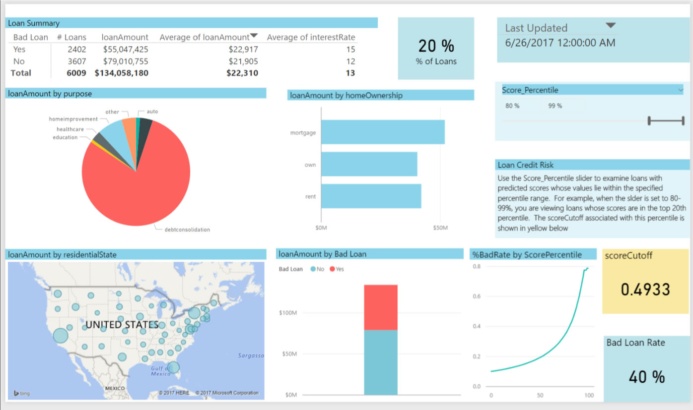 The output scores from the model have been binned according to the percentiles: the higher the percentile, and the most likely the risk of default. Bernie uses the slider showing these percentiles at the top right to find a suitable level of risk for extending a loan. He sets the slider to 80-99 to show the top 20% of scores. The cutpoint value for this is shown in yellow and he uses this score cutpoint to classify new loans - predicted scores higher than this number will be rejected.
The Loan Summary table divides those loans classified as bad in two: those that were indeed bad (Bad Loan = Yes) and those that were in fact good although they were classified as bad (Bad Loan = No). For each of those 2 categories, the table shows the number, total and average amount, and the average interest rate of the loans. This allows you to see the expected impact of choosing this cutoff value.
New Loans Tab
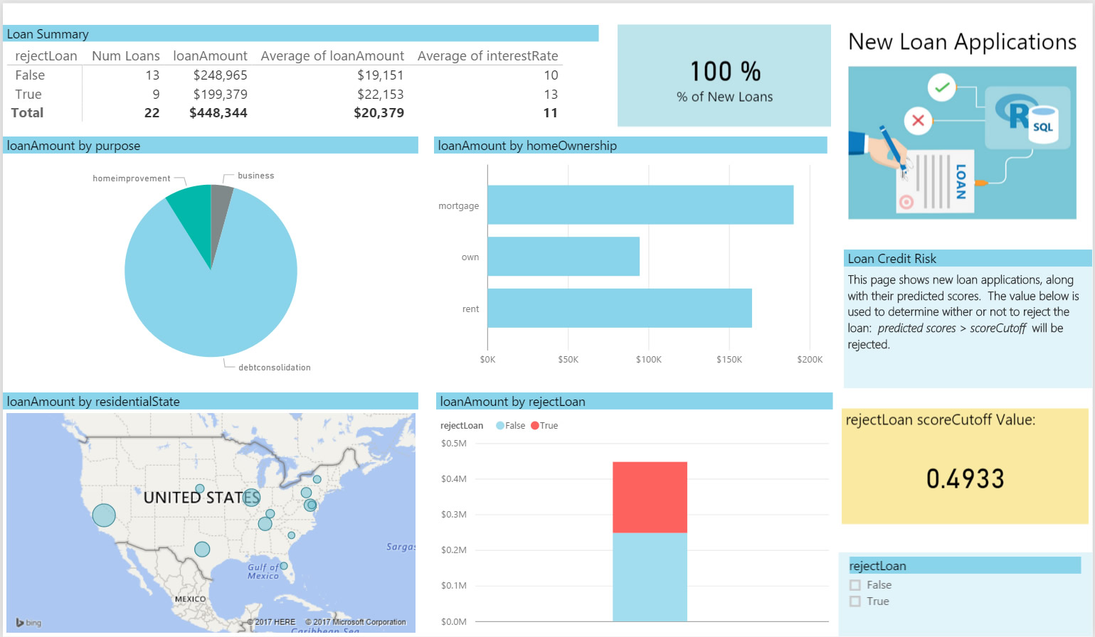 Now Bernie switches to the New Loans tab to view some scored potential loans. He uses the cutoff value from the first tab and views information about these loans. He sees he will reject 9 of the 22 potential loans based on this critera.