DecoupledClass

This class implements techniques for learning different estimators (models) for different cohorts based on the approach presented in “Decoupled classifiers for group-fair and efficient machine learning.” Cynthia Dwork, Nicole Immorlica, Adam Tauman Kalai, and Max Leiserson. Conference on fairness, accountability and transparency. PMLR, 2018. The approach searches and combines cohort-specific classifiers to optimize for different definitions of group fairness and can be used as a post-processing step on top of any model class. The current implementation in this library supports only binary classification and we welcome contributions that can extend these ideas for multi-class and regression problems.

The basis decoupling algorithm can be summarized in two steps:

• A different family of classifiers is trained on each cohort of interest. The algorithm partitions the training data for each cohort and learns a classifier for each cohort. Each cohort-specific trained classifier results in a family of potential classifiers to be used after the classifier output is adjusted based on different thresholds on the model output. For example, depending on which errors are most important to the application (e.g. false positives vs. false negatives for binary classification), thresholding the model prediction at different values of the model output (e.g. likelihood, softmax) will result in different classifiers. This step generates a whole family of classifiers based on different thresholds.

• Among the cohort-specific classifiers search for one representative classifier for each cohort such that a joint loss is optimized. This step searches through all combinations of classifiers from the previous step to find the combination that best optimizes a definition of a joint loss across all cohorts. While there are different definitions of such a joint loss, this implementation currently supports definitions of the Balanced Loss, L1 loss, and Demographic Parity as examples of losses that focus on group fairness. More definitions of losses are described in the longer version of the paper.

One issue that arises commonly in cohort-specific learning is that some cohorts may also have little data in the training set, which may hinder the capability of a decoupled classifier to learn a better estimator for that cohort. To mitigate the problem, the DecoupledClassifier class also allows using transfer learning from the overall data for these cohorts.

The figure below shows the types of scenarios that the DecoupledClassifier class can implement and how it compares to the CohortManager class. First, while the CohortManager class offers a general way to customize pipelines or train custom classifiers for cohorts, it does not offer any post-training capabilities for selecting classifiers such that they optimize a joint loss function for group fairness. In addition, transfer learning for minority cohorts is only available in the DecoupledClassifier class. To implement a scenario where the same type of data processing mitigation is applied to different cohorts separately, one can use the DecoupledClassifier with a transform pipeline (including the estimator).

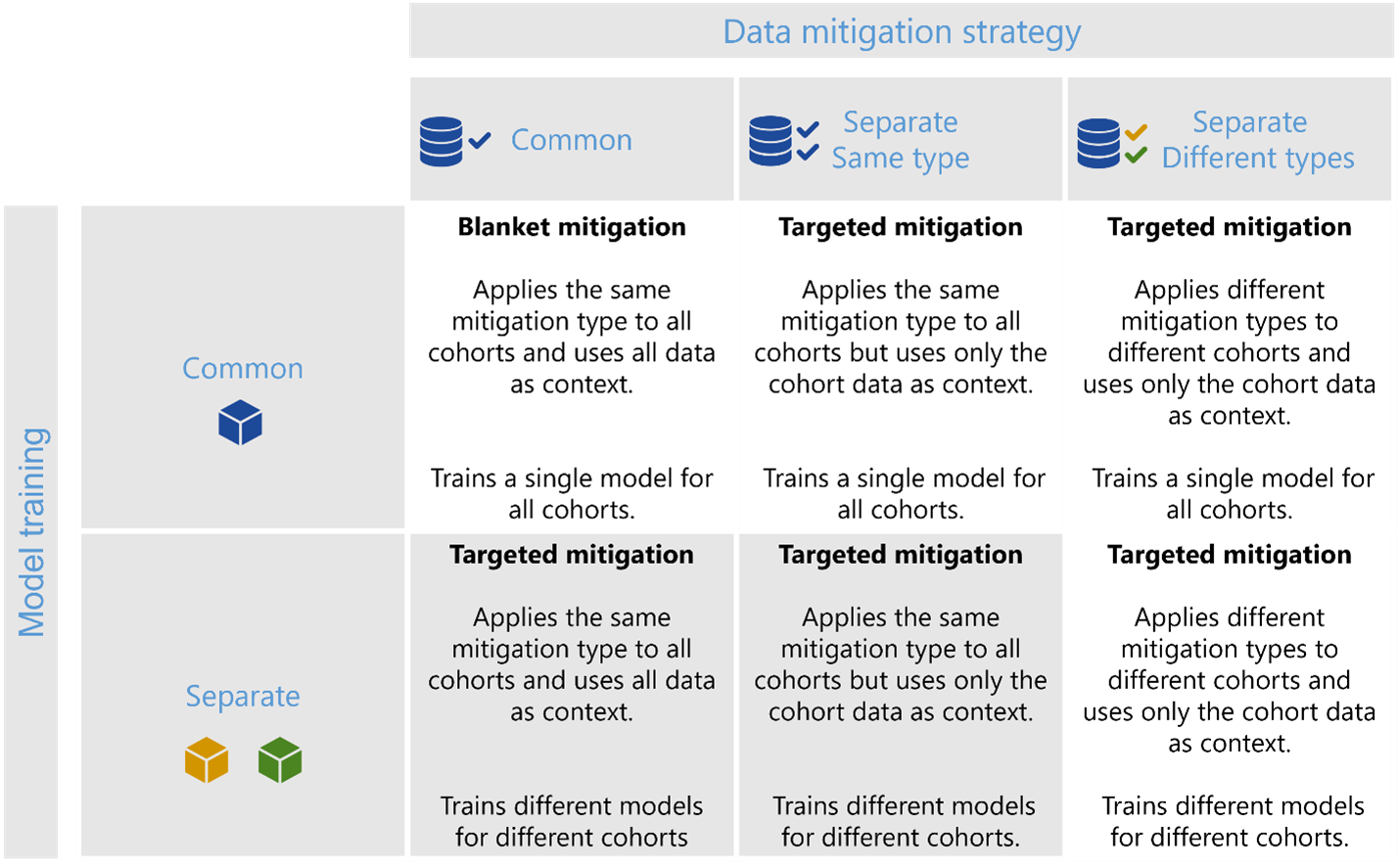
Figure 1 - The DecoupledClassifier class can currently implement the highlighted scenarios in this figure, with additional functionalities in comparison to the CohortManager being i) joint optimization of a loss function for group fairness, and ii) transfer learning for minority cohorts.

The tutorial notebook in addition to the decoupled classifiers case study notebooks demonstrate different scenarios where one can use this class.

class raimitigations.cohort.DecoupledClass(df: Optional[DataFrame] = None, label_col: Optional[str] = None, X: Optional[DataFrame] = None, y: Optional[DataFrame] = None, transform_pipe: Optional[list] = None, regression: Optional[bool] = None, cohort_def: Optional[dict] = None, cohort_col: Optional[list] = None, cohort_json_files: Optional[list] = None, theta: Union[float, List[float], bool] = False, default_theta: Optional[float] = None, cohort_dist_th: float = 0.8, min_fold_size_theta: int = 20, valid_k_folds_theta: List[int] = [3, 4, 5], estimator: Optional[BaseEstimator] = None, min_cohort_size: int = 50, min_cohort_pct: float = 0.1, minority_min_rate: float = 0.1, fairness_loss: Optional[str] = None, lambda_coef: float = 0.8, max_joint_loss_time: float = 50, verbose: bool = True)

Concrete class that trains different models over different subsets of data (cohorts). Based on the work presented in the following paper: Decoupled classifiers for group-fair and efficient machine learning. This is useful when a given cohort behaves differently from the rest of the dataset, or when a cohort represents a minority group that is underrepresented. For small cohorts, it is possible to train a model using the data of other cohorts (outside data) with a smaller weight theta (only works with models that accept instance weights). This process is herein called Transfer Learning. Instead of using transfer learning, it is also possible to merge small cohorts together, resulting in a set of sufficiently large cohorts.

Parameters

• df – the data frame to be used during the fit method. This data frame must contain all the features, including the label column (specified in the ‘label_col’ parameter). This parameter is mandatory if ‘label_col’ is also provided. The user can also provide this dataset (along with the ‘label_col’) when calling the fit() method. If df is provided during the class instantiation, it is not necessary to provide it again when calling fit(). It is also possible to use the ‘X’ and ‘y’ instead of ‘df’ and ‘label_col’, although it is mandatory to pass the pair of parameters (X,y) or (df, label_col) either during the class instantiation or during the fit() method;

• label_col – the name or index of the label column. This parameter is mandatory if ‘df’ is provided;

• X – contains only the features of the original dataset, that is, does not contain the label column. This is useful if the user has already separated the features from the label column prior to calling this class. This parameter is mandatory if ‘y’ is provided;

• y – contains only the label column of the original dataset. This parameter is mandatory if ‘X’ is provided;

• transform_pipe – a list of transformations to be used as a pre-processing pipeline. Each transformation in this list must be a valid subclass of the current library (EncoderOrdinal, BasicImputer, etc.). Some feature selection methods require a dataset with no categorical features or with no missing values (depending on the approach). If no transformations are provided, a set of default transformations will be used, which depends on the feature selection approach (subclass dependent);

• regression – if True and no estimator is provided, then create a default regression model. If False, a classifier is created instead. This parameter is ignored if an estimator is provided using the ‘estimator’ parameter;

• cohort_def – a list of cohort definitions or a dictionary of cohort definitions. A cohort condition is the same variable received by the cohort_definition parameter of the CohortDefinition class. When using a list of cohort definitions, the cohorts will be named automatically. For the dictionary of cohort definitions, the key used represents the cohort’s name, and the value assigned to each key is given by that cohort’s conditions. This parameter can’t be used together with the cohort_col parameter. Only one these two parameters must be used at a time;

• cohort_col – a list of column names that indicates which columns should be used to create a cohort. For example, if cohort_col = [“C1”, “C2”], then we first identify all possible values for column “C1” and “C2”. Suppose that the unique values in “C1” are: [0, 1, 2], and the unique values in “C2” are: [‘a’, ‘b’]. Then, we create one cohort for each combination between these two sets of unique values. This way, the first cohort will be conditioned to instances where (“C1” == 0 and “C2” == ‘a’), cohort 2 will be conditioned to (“C1” == 0 and “C2” == ‘b’), and so on. They are called the baseline cohorts. We then check if there are any of the baseline cohorts that are invalid, where an invalid cohort is considered as being a cohort with size < max(min_cohort_size, df.shape[0] * min_cohort_pct) or a cohort with a minority class (the label value with least occurrences) with an occurrence rate < minority_min_rate. Every time an invalid cohort is found, we merge this cohort to the current smallest cohort. This is simply a heuristic, as identifying the best way to merge these cohorts in a way that results in a list of valid cohorts is a complex problem that we do not try to solve here. Note that if using transfer learning (check the theta parameter for more details), then the baseline cohorts are not merged if they are found invalid. Instead, we use transfer learning over the invalid cohorts;

• cohort_json_files – a list with the name of the JSON files that contains the definition of each cohort. Each cohort is saved in a single JSON file, so the length of the cohort_json_files should be equal to the number of cohorts to be used.

• theta –

  the theta parameter is used in the transfer learning step of the decoupled classifier, and it represents the weight assigned to the instances from the outside data (data not from the current cohort) when fitting an estimator for a given cohort. The theta parameter must be a value between [0, 1], or a list of floats, or a boolean value (more information on each type ahead). This parameter is associated to how the theta is set. When a cohort with a size smaller than the minimum size allowed is found, transfer learning is used to fix this issue. Here, transfer learning occurs when a set of data not belonging to a given cohort is used when fitting that cohort’s estimator, but the instances from the outside data are assigned a smaller weight equal to theta. This weight can be fixed for all cohorts (when theta is a simple float value) or it can be identified automatically for each cohort separately (only for those cohorts that require transfer learning)(when theta is a list of floats or a boolean value). The theta parameter can be a float, a list of floats, or a boolean value. Each of the possible values is explained as follows:

  • float: the exact value assigned to the theta parameter for all cohorts. Must be a value between [0, 1];

  • list of float: a list of possible values for theta. All values in this list must be values between [0, 1]. When a cohort uses transfer learning, Cross-Validation is used with the cohort data plus the outside data using different values of theta (the values within the list of floats), and the final theta is selected as being the one associated with the highest performance in the Cross-Validation process. The Cross-Validation (CV) here splits the cohort data into K folds (the best K value is identified according to the possible values in valid_k_folds_theta), and then proceeds to use one of the folds as the test set, and the remaining folds plus the outside data as the train set. A model is fitted for the train set and then evaluated in the test set. The ROC AUC metric is obtained for each CV run until all folds have been used as a test set. We then compute the average ROC AUC score for the K runs and that gives the CV score for a given theta value. This is repeated for all possible theta values (the theta list), and the theta with the best score is selected for that cohort. This process is repeated for each cohort that requires transfer learning;

  • boolean: similar to when theta is a list of floats, but here, instead of receiving the list of possible theta from the user, a default list of possible values is used (self.THETA_VALUES). If True, uses transfer learning over small cohorts, and for each small cohort, select the best theta among the values in THETA_VALUES. If False, don’t use transfer learning;

• default_theta – the default value for theta when a given cohort is too small to use Cross-Validation to find the best theta value among a list of possible values. This parameter is only used when the ‘theta’ parameter is True or a list of float values. When splitting a cohort into K folds, each fold must have a minimum size according to the min_fold_size_theta parameter. When that is not possible, we reduce the value of K (according to the possible values of K specified in the valid_k_folds_theta parameter) and test if now we can split the cohort into K folds, each fold being larger than min_fold_size_theta. We do this until all K values are tested, and if none of these results in folds large enough, a default value of theta is used to avoid raising an error. This default value is given by this parameter. If None, then don’t use any default value in these cases. Instead, raise an error;

• cohort_dist_th – a value between [0, 1] that represents the threshold used to determine if the label distribution of two cohorts are similar or not. If the distance between these two distributions is <= cohort_dist_th, then the cohorts are considered compatible, and considered incompatible otherwise. This is used to determine how to build the outside data used for transfer learning: when a cohort uses transfer learning (check the parameter ‘theta’ for more information on that process), the outside data used for it must be comprised of data from other cohorts that follow a somehow similar label distribution. Otherwise, the use of outside data could be more harmful than useful. Therefore, for each cohort using transfer learning, we check which other cohorts have a similar label distribution. The similarity of these distributions is computed using the Jensen-Shanon distance, which computes the distance between two distributions. This distance returns a value between [0, 1], where values close to 0 mean that two distributions being compared are similar, while values close to 1 mean that these distributions are considerably different. If the distance between the label distribution of both cohorts is smaller than a provided threshold (cohort_dist_th), then the outside cohort is considered compatible with the current cohort;

• min_fold_size_theta – the minimum size allowed for each fold when doing Cross-Validation to determine the best value for theta. For more information, check the parameter default_theta;

• valid_k_folds_theta – a list of possible values for K, which represents the number of splits used over a cohort data when doing Cross-Validation (to determine the best theta value). The last value in this list is used, and if this K value results in invalid folds, the second-to-last value in the list is. This process goes on until a valid K value is found in the list. We recommend filling this list with increasing values of K. This way, the largest valid value of K will be selected; For more information, check the parameter default_theta;

• estimator – the estimator used for each cohort. Each cohort will have their own copy of this estimator, which means that different instances of the same estimator is used for each cohort;

• min_cohort_size – the minimum size a cohort is allowed to have to be considered valid. Check the cohort_col parameter for more information;

• min_cohort_pct – a value between [0, 1] that determines the minimum size allowed for a cohort. The minimum size is given by the size of the full dataset (df.shape[0]) multiplied by min_cohort_pct. The maximum value between min_cohort_size and (df.shape[0] * min_cohort_pct) is used to determine the minimum size allowed for a cohort. Check the cohort_col parameter for more information;

• fairness_loss –

  The fairness loss that should be optimized alongside the L1 loss. This is only possible for binary classification problems. For regression or multi-class problems, this parameter should be set to None (default value), otherwise, an error will be raised. The L1 and fairness losses are computed over the binarized predictions, not over the probabilities. Therefore, the decoupled classifier tries to identify the best set of thresholds (one for each estimator, where we have one estimator for each cohort) that produces the lowest joint loss (L1 + fairness loss). There are 3 available fairness losses:

  • None: don’t use any fairness loss. The threshold used for each cohort is identified through the ROC curve, that is, doesn’t consider any fairness metric. This is the default behavior;

  • ”balanced”: the Balanced loss is computed as the mean loss value over the L1 loss of each cohort. This loss is useful when we want that all cohorts to have a similar L1 loss, where all cohorts are considered with an equal weight, which makes it ideal for unbalanced datasets;

  • ”num_parity”: the Numerical Parity loss forces all cohorts to have a similar number of positive labels. This loss is useful in a situation where a model should output an equal number of positive labels for each cohort;

  • ”dem_parity”: the Demographic Parity loss forces all cohorts to have a similar rate of positive labels. This is somehow similar to the Numerical Parity loss, but this loss accounts for the difference in size of each cohort, that is, the number of positive labels should be different for cohorts with different sizes, but the ratio of positive labels over the size of the cohort should be consistent across cohorts. This is useful when we want an unbiased model, that is, a model that outputs an equal proportion of positive labels without considering the cohort to which an instance belongs to;

  Note: optimizing the threshold values for each cohort according to a fairness loss can take a considerable time depending on the size of the dataset. Check the max_joint_loss_time parameter to learn how to control the allowed time for computing these thresholds;

• lambda_coef –

  the weight assigned to the L1 loss when computing the joint loss (L1 + fairness loss). This parameter is ignored when fairness_loss = None. When fairness != None, after the estimator of each cohort is fitted, we optimize the thresholds used to binarize the final predictions according to the following loss function:

  \[\hat{L} = \lambda L_{1} + (1-\lambda) L_{fair}\]

  where:

  • L_1 is the L1 loss function over the binarized predictions

  • L_{fair} is the fairness loss being used

  The L_1 loss tends to have smaller values than the fairness losses, so we recommend trying larger values for the lambda_coef parameter, otherwise, the thresholds might look only to the fairness loss;

• max_joint_loss_time – the maximum time (in seconds) allowed for the decoupled classifier to run its fairness optimization step. This parameter is ignored when fairness_loss = None. When fairness != None, the decoupled classifier will try to find the best set of thresholds to be used for each cohort such that the final predictions result in a minimum joint loss. However, this optimization step is computationally expensive, and can take some time to be finalized depending on the number of cohorts and the size of the dataset. To avoid long execution times, we can specify the maximum time allowed for the decoupled classifier to run this step. If the optimization step reaches the maximum time, then the best set of thresholds found so far is returned;

• minority_min_rate – the minimum occurrence rate for the minority class (from the label column) that a cohort is allowed to have. If the minority class of the cohort has an occurrence rate lower than min_rate, the cohort is considered invalid. Check the cohort_col parameter for more information;

• verbose – indicates whether internal messages should be printed or not.

fit(X: Optional[Union[DataFrame, ndarray]] = None, y: Optional[Union[Series, ndarray]] = None, df: Optional[DataFrame] = None, label_col: Optional[str] = None)

Overwrites the fit() method of the base CohortHandler class. Implements the steps for running the fit method for the current class.

Parameters

• X – contains only the features of the original dataset, that is, does not contain the label column;

• y – contains only the label column of the original dataset;

• df – the full dataset;

• label_col – the name or index of the label column;

Check the documentation of the _set_df_mult method (DataProcessing class) for more information on how these parameters work.

get_threasholds_dict()

Returns a dictionary containing the best threshold value found for the estimator of each cohort.

predict(X: Union[DataFrame, ndarray], split_pred: bool = False)

Calls the transform() method of all transformers in all pipelines, followed by the predict() method for the estimator.

Parameters

• X – contains only the features of the dataset to be transformed;

• split_pred – if True, return a dictionary with the predictions for each cohort. If False, return a single predictions array;

Returns

an array with the predictions of all instances of the dataset, built from the predictions of each cohort, or a dictionary with the predictions for each cohort;

Return type

np.ndarray or dict

predict_proba(X: Union[DataFrame, ndarray], split_pred: bool = False)

Calls the transform() method of all transformers in all pipelines, followed by the predict_proba() method for the estimator.

Parameters

• X – contains only the features of the dataset to be transformed;

• split_pred – if True, return a dictionary with the predictions for each cohort. If False, return a single predictions array;

Returns

an array with the predictions of all instances of the dataset, built from the predictions of each cohort, or a dictionary with the predictions for each cohort;

Return type

np.ndarray or dict

print_cohorts()

Print the information of all cohorts created.

Class Diagram

Examples

Decoupled Classifiers

Decoupled Classifiers Case Study 1

Decoupled Classifiers Case Study 2

Decoupled Classifiers Case Study 3