Decoupled Classifiers Case Study 2

This notebook will follow a similar approach to what was done in the notebook Decoupled Classifiers Case Study 1, but this time we’ll use a real dataset.

import sys
sys.path.append('../../../../notebooks')

import pandas as pd
import numpy as np
import random

from sklearn.tree import DecisionTreeClassifier
from lightgbm import LGBMClassifier

from raimitigations.utils import split_data
import raimitigations.dataprocessing as dp
from raimitigations.cohort import DecoupledClass, CohortDefinition, CohortManager, fetch_cohort_results, plot_value_counts_cohort
from sklearn.pipeline import Pipeline
from download import download_datasets

SEED = 100

Load and split the data into train and test sets:

data_dir = "../../../../datasets/census/"
download_datasets(data_dir)

label_col = "income"
df_train = pd.read_csv(data_dir + "train.csv")
df_test = pd.read_csv(data_dir + "test.csv")
# convert to 0 and 1 encoding
df_train[label_col] = df_train[label_col].apply(lambda x: 0 if x == "<=50K" else 1)
df_test[label_col] = df_test[label_col].apply(lambda x: 0 if x == "<=50K" else 1)

X_train = df_train.drop(columns=[label_col])
y_train = df_train[label_col]
X_test = df_test.drop(columns=[label_col])
y_test = df_test[label_col]

df_train

	income	age	workclass	fnlwgt	education	education-num	marital-status	occupation	relationship	race	gender	capital-gain	capital-loss	hours-per-week	native-country
0	0	39	State-gov	77516	Bachelors	13	Never-married	Adm-clerical	Not-in-family	White	Male	2174	0	40	United-States
1	0	50	Self-emp-not-inc	83311	Bachelors	13	Married-civ-spouse	Exec-managerial	Husband	White	Male	0	0	13	United-States
2	0	38	Private	215646	HS-grad	9	Divorced	Handlers-cleaners	Not-in-family	White	Male	0	0	40	United-States
3	0	53	Private	234721	11th	7	Married-civ-spouse	Handlers-cleaners	Husband	Black	Male	0	0	40	United-States
4	0	28	Private	338409	Bachelors	13	Married-civ-spouse	Prof-specialty	Wife	Black	Female	0	0	40	Cuba
...	...	...	...	...	...	...	...	...	...	...	...	...	...	...	...
32556	0	27	Private	257302	Assoc-acdm	12	Married-civ-spouse	Tech-support	Wife	White	Female	0	0	38	United-States
32557	1	40	Private	154374	HS-grad	9	Married-civ-spouse	Machine-op-inspct	Husband	White	Male	0	0	40	United-States
32558	0	58	Private	151910	HS-grad	9	Widowed	Adm-clerical	Unmarried	White	Female	0	0	40	United-States
32559	0	22	Private	201490	HS-grad	9	Never-married	Adm-clerical	Own-child	White	Male	0	0	20	United-States
32560	1	52	Self-emp-inc	287927	HS-grad	9	Married-civ-spouse	Exec-managerial	Wife	White	Female	15024	0	40	United-States

32561 rows × 15 columns

def get_model():
    #model = DecisionTreeClassifier(max_features="sqrt")
    model = LGBMClassifier(random_state=SEED)
    return model

Taking a closer look at a few sensitive attributes of this dataset and possible imbalance in the data.

The “race” cohorts

Let’s start by plotting the label distribution over the “race” cohorts.

# BASELINE: "race"
cohort_set = CohortManager(
    transform_pipe=[
        dp.DataStandardScaler(verbose=False),
        dp.EncoderOHE(drop=False, unknown_err=False, verbose=False),
        get_model()
    ],
    cohort_col=["race"]
)
cohort_set.fit(X=X_train, y=y_train)
subsets = cohort_set.get_subsets(X_train, y_train, apply_transform=False)

print(y_train.value_counts())

for key in subsets.keys():
    print(f"\n{key} : {cohort_set.get_queries()[key]}:\n{subsets[key]['y'].value_counts()}\n***********")

plot_value_counts_cohort(y_train, subsets, normalize=False)

0    24720
1     7841
Name: income, dtype: int64

cohort_0 : (`race` == " Amer-Indian-Eskimo"):
0    275
1     36
Name: income, dtype: int64
***********

cohort_1 : (`race` == " Asian-Pac-Islander"):
0    763
1    276
Name: income, dtype: int64
***********

cohort_2 : (`race` == " Black"):
0    2737
1     387
Name: income, dtype: int64
***********

cohort_3 : (`race` == " Other"):
0    246
1     25
Name: income, dtype: int64
***********

cohort_4 : (`race` == " White"):
0    20699
1     7117
Name: income, dtype: int64
***********

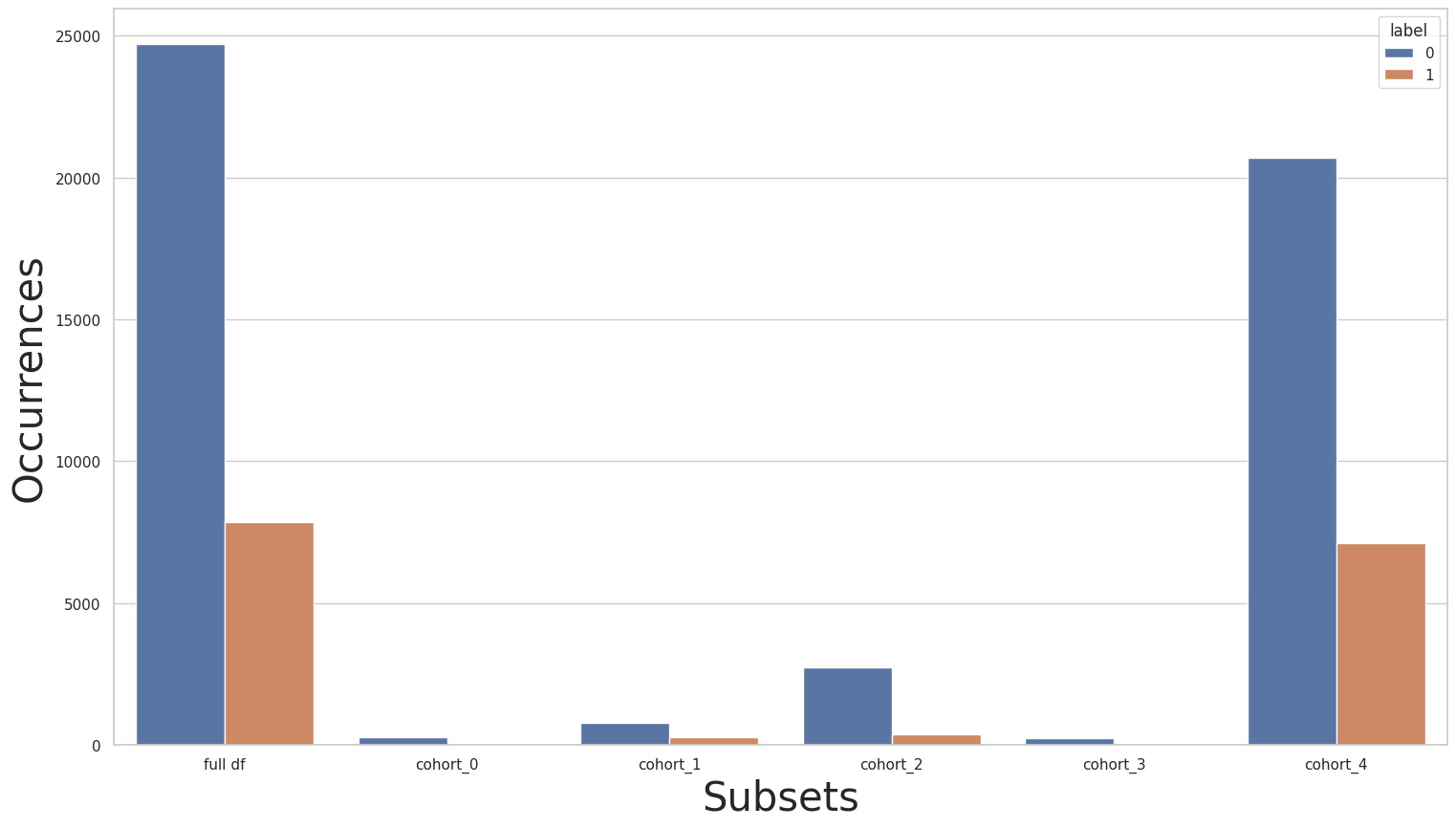
Clearly, we can see an imbalance in the size of cohorts and label distribution. Given the sensitivity of the “race” attribute, merging cohorts might not be an appropriate solution, instead, let’s take a look at the effect of transfer learning:

Transfer Learning

Note: the following experiment is expected to fail. We’ll explain why it failed in the following cells

preprocessing = [dp.DataStandardScaler(verbose=False), dp.EncoderOHE(drop=False, unknown_err=False, verbose=False)]

dec_class = DecoupledClass(
    cohort_col=["race"],
    theta=True,
    min_fold_size_theta=15,
    min_cohort_pct=0.1,
    minority_min_rate=0.1,
    transform_pipe=preprocessing,
    estimator=get_model()
)
try:
    dec_class.fit(X_train, y_train)
except Exception as e:
    print(e)

INVALID COHORTS:
cohort_3:
        Size: 271
        Query:
                (`race` == " Other")
        Value Counts:
                0: 246 (90.77%)
                1: 25 (9.23%)
        Invalid: False
ERROR: Cannot use transfer learning over cohorts with skewed distributions.

The above code fails because one or more dataset has a label distribution invalidity, meaning that at least one cohort doesn’t satisfy the minimum rate requirement of the minority class. In order to try and solve this skewed distribution, we can use the Rebalance functionality of this library to re-balance the data.

c0_pipe = [dp.Rebalance(strategy_over=0.5, verbose=False)]
c1_pipe = []
c2_pipe = []
c3_pipe = [dp.Rebalance(strategy_over=0.5, verbose=False)]
c4_pipe = []

cohort_set = CohortManager(
    transform_pipe=[c0_pipe, c1_pipe, c2_pipe, c3_pipe, c4_pipe],
    cohort_col=["race"]
)

rebalanced_X_train, rebalanced_y_train = cohort_set.fit_resample(X=X_train, y=y_train)

/home/mmendonca/anaconda3/envs/raipub/lib/python3.9/site-packages/sklearn/preprocessing/_encoders.py:808: FutureWarning: `sparse` was renamed to `sparse_output` in version 1.2 and will be removed in 1.4. `sparse_output` is ignored unless you leave `sparse` to its default value.
  warnings.warn(
/home/mmendonca/anaconda3/envs/raipub/lib/python3.9/site-packages/sklearn/preprocessing/_encoders.py:808: FutureWarning: `sparse` was renamed to `sparse_output` in version 1.2 and will be removed in 1.4. `sparse_output` is ignored unless you leave `sparse` to its default value.
  warnings.warn(

let’s look at the label distribution plots of the rebalanced data:

cohort_set = CohortManager(
    transform_pipe=[
        dp.DataStandardScaler(verbose=False),
        dp.EncoderOHE(drop=False, unknown_err=False, verbose=False),
        get_model()
    ],
    cohort_col=["race"]
)
cohort_set.fit(X=rebalanced_X_train, y=rebalanced_y_train)
subsets = cohort_set.get_subsets(rebalanced_X_train, rebalanced_y_train, apply_transform=False)

print(rebalanced_y_train.value_counts())

for key in subsets.keys():
    print(f"\n{key} : {cohort_set.get_queries()[key]}:\n{subsets[key]['y'].value_counts()}\n***********")

plot_value_counts_cohort(rebalanced_y_train, subsets, normalize=False)

0    24720
1     8040
Name: income, dtype: int64

cohort_0 : (`race` == " Amer-Indian-Eskimo"):
0    275
1    137
Name: income, dtype: int64
***********

cohort_1 : (`race` == " Asian-Pac-Islander"):
0    763
1    276
Name: income, dtype: int64
***********

cohort_2 : (`race` == " Black"):
0    2737
1     387
Name: income, dtype: int64
***********

cohort_3 : (`race` == " Other"):
0    246
1    123
Name: income, dtype: int64
***********

cohort_4 : (`race` == " White"):
0    20699
1     7117
Name: income, dtype: int64
***********

then the performance metrics of the rebalanced baseline cohorts:

pred_cht = cohort_set.predict_proba(X_test)

pred_train = cohort_set.predict_proba(rebalanced_X_train)
metrics_train, th_dict = fetch_cohort_results(rebalanced_X_train, rebalanced_y_train, pred_train, cohort_col=["race"], return_th_dict=True)
fetch_cohort_results(X_test, y_test, pred_cht, cohort_col=["race"], fixed_th=th_dict)

	cohort	cht_query	roc	precision	recall	f1	accuracy	threshold	num_pos	%_pos	cht_size
0	all	all	0.919891	0.779694	0.836502	0.798674	0.838585	0.260096	5186	0.318531	16281
1	cohort_0	(`race` == " Amer-Indian-Eskimo")	0.719173	0.736372	0.594549	0.623024	0.886792	0.730358	7	0.044025	159
2	cohort_1	(`race` == " Asian-Pac-Islander")	0.881606	0.795724	0.750569	0.767495	0.827083	0.522477	104	0.216667	480
3	cohort_2	(`race` == " Black")	0.920955	0.771581	0.767609	0.769573	0.907111	0.367778	176	0.112748	1561
4	cohort_3	(`race` == " Other")	0.906909	0.839147	0.595455	0.617357	0.844444	0.943149	6	0.044444	135
5	cohort_4	(`race` == " White")	0.924379	0.780414	0.839327	0.797787	0.830346	0.254678	4860	0.348487	13946

And now let’s attempt transfer learning again using the rebalanced data:

preprocessing = [dp.DataStandardScaler(verbose=False), dp.EncoderOHE(drop=False, unknown_err=False, verbose=False)]

dec_class = DecoupledClass(
    cohort_col=["race"],
    theta=0.8,
    min_fold_size_theta=15,
    min_cohort_pct=0.1,
    minority_min_rate=0.1,
    transform_pipe=preprocessing,
    estimator=get_model()
)
dec_class.fit(rebalanced_X_train, rebalanced_y_train)

dec_class.print_cohorts()

subsets = dec_class.get_subsets(rebalanced_X_train, rebalanced_y_train, apply_transform=True)

print(rebalanced_y_train.value_counts())

for key in subsets.keys():
    print(f"\n{key} : {dec_class.get_queries()[key]}:\n{subsets[key]['y'].value_counts()}\n***********")

plot_value_counts_cohort(rebalanced_y_train, subsets, normalize=False)

FINAL COHORTS
cohort_0:
        Size: 412
        Query:
                (`race` == " Amer-Indian-Eskimo")
        Value Counts:
                0: 275 (66.75%)
                1: 137 (33.25%)
        Invalid: True
                Cohorts used as outside data: ['cohort_1', 'cohort_2', 'cohort_3', 'cohort_4']
                Theta = 0.8


cohort_1:
        Size: 1039
        Query:
                (`race` == " Asian-Pac-Islander")
        Value Counts:
                0: 763 (73.44%)
                1: 276 (26.56%)
        Invalid: True
                Cohorts used as outside data: ['cohort_0', 'cohort_2', 'cohort_3', 'cohort_4']
                Theta = 0.8


cohort_2:
        Size: 3124
        Query:
                (`race` == " Black")
        Value Counts:
                0: 2737 (87.61%)
                1: 387 (12.39%)
        Invalid: True
                Cohorts used as outside data: ['cohort_0', 'cohort_1', 'cohort_3', 'cohort_4']
                Theta = 0.8


cohort_3:
        Size: 369
        Query:
                (`race` == " Other")
        Value Counts:
                0: 246 (66.67%)
                1: 123 (33.33%)
        Invalid: True
                Cohorts used as outside data: ['cohort_0', 'cohort_1', 'cohort_2', 'cohort_4']
                Theta = 0.8


cohort_4:
        Size: 27816
        Query:
                (`race` == " White")
        Value Counts:
                0: 20699 (74.41%)
                1: 7117 (25.59%)
        Invalid: False


0    24720
1     8040
Name: income, dtype: int64

cohort_0 : (`race` == " Amer-Indian-Eskimo"):
0    275
1    137
Name: income, dtype: int64
***********

cohort_1 : (`race` == " Asian-Pac-Islander"):
0    763
1    276
Name: income, dtype: int64
***********

cohort_2 : (`race` == " Black"):
0    2737
1     387
Name: income, dtype: int64
***********

cohort_3 : (`race` == " Other"):
0    246
1    123
Name: income, dtype: int64
***********

cohort_4 : (`race` == " White"):
0    20699
1     7117
Name: income, dtype: int64
***********

th_dict = dec_class.get_threasholds_dict()
pred = dec_class.predict_proba(X_test)
fetch_cohort_results(X_test, y_test, pred, cohort_def=dec_class, fixed_th=th_dict)

	cohort	cht_query	roc	precision	recall	f1	accuracy	threshold	num_pos	%_pos	cht_size
0	all	all	0.927809	0.835215	0.799236	0.814789	0.873288	0.500000	3285	0.201769	16281
1	cohort_0	(`race` == " Amer-Indian-Eskimo")	0.941729	0.799934	0.839850	0.817998	0.918239	0.406598	22	0.138365	159
2	cohort_1	(`race` == " Asian-Pac-Islander")	0.905202	0.793487	0.802702	0.797815	0.835417	0.408684	140	0.291667	480
3	cohort_2	(`race` == " Black")	0.950893	0.834517	0.809811	0.821497	0.930173	0.404750	164	0.105061	1561
4	cohort_3	(`race` == " Other")	0.973455	0.877273	0.877273	0.877273	0.925926	0.395015	25	0.185185	135
5	cohort_4	(`race` == " White")	0.924379	0.805904	0.820844	0.812812	0.856016	0.384067	3756	0.269325	13946

…thanks to the rebalance, we were able to run transfer learning over the “race” cohorts.

It seems that transfer learning has a positive effect on most cohorts in the test set. We can see improvement in the ROC metric, label distribution and performance with a generally more comparable distribution among cohorts.

The “gender” cohorts

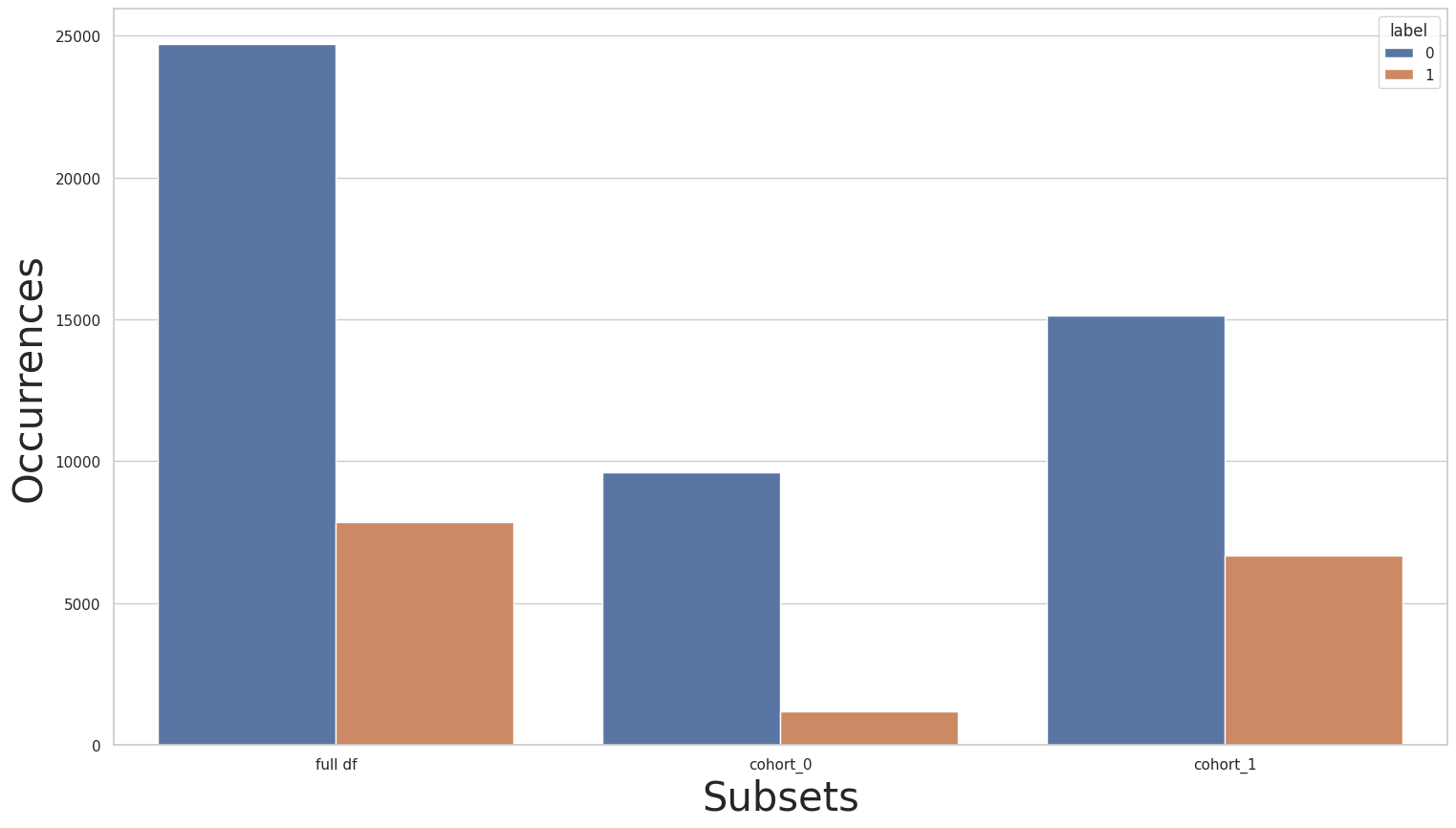
Secondly, let’s look at the plots and label distribution of another sensitive attribute:

cohort_set = CohortManager(
    transform_pipe=[
        dp.DataStandardScaler(verbose=False),
        dp.EncoderOHE(drop=False, unknown_err=False, verbose=False),
        get_model()
    ],
    cohort_col=["gender"]
)
cohort_set.fit(X=X_train, y=y_train)
subsets = cohort_set.get_subsets(X_train, y_train, apply_transform=False)

print(y_train.value_counts())

for key in subsets.keys():
    print(f"\n{key} : {cohort_set.get_queries()[key]}:\n{subsets[key]['y'].value_counts()}\n***********")

plot_value_counts_cohort(y_train, subsets, normalize=False)

0    24720
1     7841
Name: income, dtype: int64

cohort_0 : (`gender` == " Female"):
0    9592
1    1179
Name: income, dtype: int64
***********

cohort_1 : (`gender` == " Male"):
0    15128
1     6662
Name: income, dtype: int64
***********

pred_cht = cohort_set.predict_proba(X_test)

pred_train = cohort_set.predict_proba(X_train)
metrics_train, th_dict = fetch_cohort_results(X_train, y_train, pred_train, cohort_col=["gender"], return_th_dict=True)
fetch_cohort_results(X_test, y_test, pred_cht, cohort_col=["gender"], fixed_th=th_dict)

	cohort	cht_query	roc	precision	recall	f1	accuracy	threshold	num_pos	%_pos	cht_size
0	all	all	0.924731	0.775651	0.840135	0.794981	0.832750	0.243250	5447	0.334562	16281
1	cohort_0	(`gender` == " Female")	0.939232	0.749313	0.854318	0.787376	0.899465	0.156009	895	0.165099	5421
2	cohort_1	(`gender` == " Male")	0.908182	0.778074	0.818033	0.787847	0.806906	0.280206	4349	0.400460	10860

The distribution of the “gender” column might not be as skewed as the “race” column, but we can still see that cohort_1 has a more balanced distribution than cohort_0. Let’s attempt to use transfer learning over these cohorts:

Transfer Learning

preprocessing = [dp.DataStandardScaler(verbose=False), dp.EncoderOHE(drop=False, unknown_err=False, verbose=False)]

dec_class = DecoupledClass(
    cohort_col=["gender"],
    theta=True,
    min_fold_size_theta=15,
    min_cohort_pct=0.1,
    minority_min_rate=0.1,
    transform_pipe=preprocessing,
    estimator=get_model()
)
dec_class.fit(X_train, y_train)

dec_class.print_cohorts()

FINAL COHORTS
cohort_0:
        Size: 10771
        Query:
                (`gender` == " Female")
        Value Counts:
                0: 9592 (89.05%)
                1: 1179 (10.95%)
        Invalid: False


cohort_1:
        Size: 21790
        Query:
                (`gender` == " Male")
        Value Counts:
                0: 15128 (69.43%)
                1: 6662 (30.57%)
        Invalid: False

th_dict = dec_class.get_threasholds_dict()
pred = dec_class.predict_proba(X_test)
fetch_cohort_results(X_test, y_test, pred, cohort_def=dec_class, fixed_th=th_dict)

	cohort	cht_query	roc	precision	recall	f1	accuracy	threshold	num_pos	%_pos	cht_size
0	all	all	0.924731	0.832133	0.794795	0.810810	0.870892	0.500000	3260	0.200233	16281
1	cohort_0	(`gender` == " Female")	0.939232	0.814410	0.824649	0.819414	0.928795	0.341452	612	0.112894	5421
2	cohort_1	(`gender` == " Male")	0.908182	0.791165	0.811141	0.799352	0.825414	0.365531	3690	0.339779	10860

In the case of the “gender” column, observing the two past results, we notice that transfer learning has improved the precision, F1 score, and accuracy for both cohorts. Therefore, transfer learning has proved useful in this scenario compared to using the more generic CohortManager approach.

Fairness Optimization

One issue we can identify on the previous result is that the rate of positive labels for cohort_0 is smaller than the positive rate in cohort_1. In some cases, this is not desirable, as this shows that the model fitted has some bias in regard to the sensitive feature (in this case, the gender column). Let’s try to mitigate this issue by using the DecoupledClass with Transfer Learning + Fairness optimization using the Demographic Parity loss.

preprocessing = [dp.DataStandardScaler(verbose=False), dp.EncoderOHE(drop=False, unknown_err=False, verbose=False)]

dec_class = DecoupledClass(
    cohort_col=["gender"],
    theta=True,
    min_fold_size_theta=15,
    min_cohort_pct=0.1,
    minority_min_rate=0.1,
    transform_pipe=preprocessing,
    fairness_loss="dem_parity",
    lambda_coef=0.3,
    max_joint_loss_time=200,
    estimator=get_model()
)
dec_class.fit(X_train, y_train)

dec_class.print_cohorts()

FINAL COHORTS
cohort_0:
        Size: 10771
        Query:
                (`gender` == " Female")
        Value Counts:
                0: 9592 (89.05%)
                1: 1179 (10.95%)
        Invalid: False


cohort_1:
        Size: 21790
        Query:
                (`gender` == " Male")
        Value Counts:
                0: 15128 (69.43%)
                1: 6662 (30.57%)
        Invalid: False

th_dict = dec_class.get_threasholds_dict()
pred = dec_class.predict_proba(X_test)
fetch_cohort_results(X_test, y_test, pred, cohort_def=dec_class, fixed_th=th_dict)

	cohort	cht_query	roc	precision	recall	f1	accuracy	threshold	num_pos	%_pos	cht_size
0	all	all	0.924731	0.832133	0.794795	0.810810	0.870892	0.500000	3260	0.200233	16281
1	cohort_0	(`gender` == " Female")	0.939232	0.643159	0.834692	0.643880	0.749124	0.023640	1884	0.347537	5421
2	cohort_1	(`gender` == " Male")	0.908182	0.791165	0.811141	0.799352	0.825414	0.365531	3690	0.339779	10860

The “relationship” cohorts

Lastly, we’ll take a closer look at the relationship column, starting with the baseline:

cohort_set = CohortManager(
    transform_pipe=[
        dp.DataStandardScaler(verbose=False),
        dp.EncoderOHE(drop=False, unknown_err=False, verbose=False),
        get_model()
    ],
    cohort_col=["relationship"]
)
cohort_set.fit(X=X_train, y=y_train)
subsets = cohort_set.get_subsets(X_train, y_train, apply_transform=False)

print(y_train.value_counts())

for key in subsets.keys():
    print(f"\n{key} : {cohort_set.get_queries()[key]}:\n{subsets[key]['y'].value_counts()}\n***********")

plot_value_counts_cohort(y_train, subsets, normalize=False)

0    24720
1     7841
Name: income, dtype: int64

cohort_0 : (`relationship` == " Husband"):
0    7275
1    5918
Name: income, dtype: int64
***********

cohort_1 : (`relationship` == " Not-in-family"):
0    7449
1     856
Name: income, dtype: int64
***********

cohort_2 : (`relationship` == " Other-relative"):
0    944
1     37
Name: income, dtype: int64
***********

cohort_3 : (`relationship` == " Own-child"):
0    5001
1      67
Name: income, dtype: int64
***********

cohort_4 : (`relationship` == " Unmarried"):
0    3228
1     218
Name: income, dtype: int64
***********

cohort_5 : (`relationship` == " Wife"):
0    823
1    745
Name: income, dtype: int64
***********

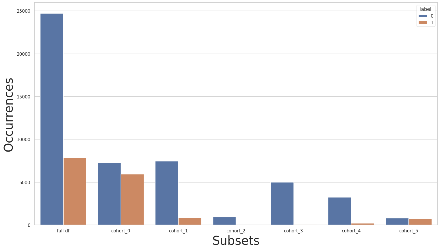
similar to the “race” column, we can see that some cohorts are smaller and with more skewness in label distribution than others. Can we apply transfer learning in this case?

Transfer Learning

preprocessing = [dp.DataStandardScaler(verbose=False), dp.EncoderOHE(drop=False, unknown_err=False, verbose=False)]

dec_class = DecoupledClass(
    cohort_col=["relationship"],
    theta=True,
    min_fold_size_theta=15,
    min_cohort_pct=0.1,
    minority_min_rate=0.1,
    transform_pipe=preprocessing,
    estimator=get_model()
)
try:
    dec_class.fit(X_train, y_train)
except Exception as e:
    print(e)

INVALID COHORTS:
cohort_2:
        Size: 981
        Query:
                (`relationship` == " Other-relative")
        Value Counts:
                0: 944 (96.23%)
                1: 37 (3.77%)
        Invalid: False
cohort_3:
        Size: 5068
        Query:
                (`relationship` == " Own-child")
        Value Counts:
                0: 5001 (98.68%)
                1: 67 (1.32%)
        Invalid: False
cohort_4:
        Size: 3446
        Query:
                (`relationship` == " Unmarried")
        Value Counts:
                0: 3228 (93.67%)
                1: 218 (6.33%)
        Invalid: False
ERROR: Cannot use transfer learning over cohorts with skewed distributions.

Similar to the “race” column, we are unable to directly apply transfer learning over these cohorts, so we will rebalance the training data first:

c0_pipe = []
c1_pipe = [dp.Rebalance(strategy_over='minority', verbose=False)]
c2_pipe = [dp.Rebalance(strategy_over='minority', verbose=False)]
c3_pipe = [dp.Rebalance(strategy_over='minority', verbose=False)]
c4_pipe = [dp.Rebalance(strategy_over='minority', verbose=False)]
c5_pipe = []

cohort_set = CohortManager(
    transform_pipe=[c0_pipe, c1_pipe, c2_pipe, c3_pipe, c4_pipe, c5_pipe],
    cohort_col=["relationship"]
)

rebalanced_X_train, rebalanced_y_train = cohort_set.fit_resample(X=X_train, y=y_train)

/home/mmendonca/anaconda3/envs/raipub/lib/python3.9/site-packages/sklearn/preprocessing/_encoders.py:808: FutureWarning: `sparse` was renamed to `sparse_output` in version 1.2 and will be removed in 1.4. `sparse_output` is ignored unless you leave `sparse` to its default value.
  warnings.warn(
/home/mmendonca/anaconda3/envs/raipub/lib/python3.9/site-packages/sklearn/preprocessing/_encoders.py:808: FutureWarning: `sparse` was renamed to `sparse_output` in version 1.2 and will be removed in 1.4. `sparse_output` is ignored unless you leave `sparse` to its default value.
  warnings.warn(
/home/mmendonca/anaconda3/envs/raipub/lib/python3.9/site-packages/sklearn/preprocessing/_encoders.py:808: FutureWarning: `sparse` was renamed to `sparse_output` in version 1.2 and will be removed in 1.4. `sparse_output` is ignored unless you leave `sparse` to its default value.
  warnings.warn(
/home/mmendonca/anaconda3/envs/raipub/lib/python3.9/site-packages/sklearn/preprocessing/_encoders.py:808: FutureWarning: `sparse` was renamed to `sparse_output` in version 1.2 and will be removed in 1.4. `sparse_output` is ignored unless you leave `sparse` to its default value.
  warnings.warn(

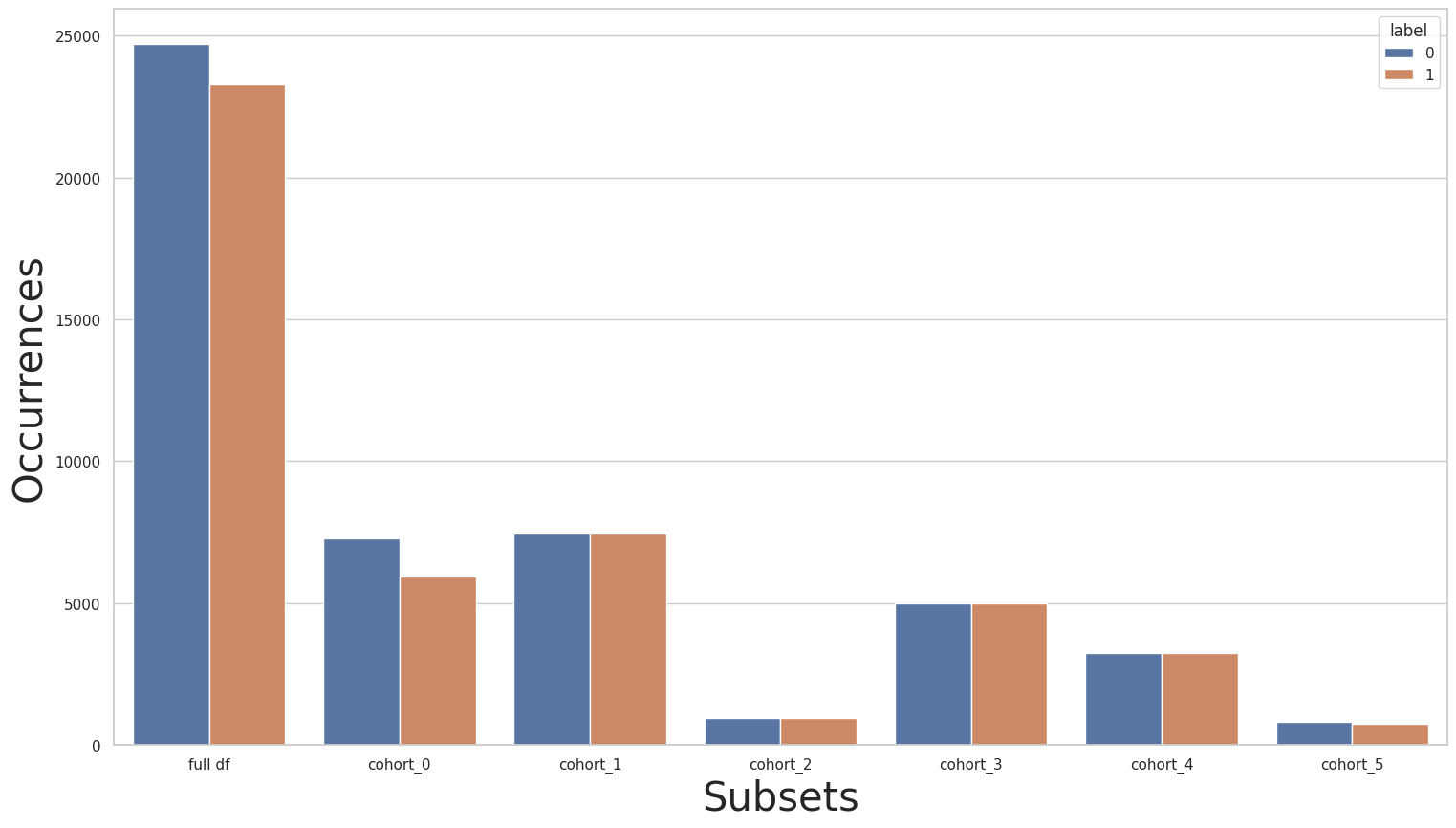
Now let’s run the baseline plots again:

cohort_set = CohortManager(
    transform_pipe=[
        dp.DataStandardScaler(verbose=False),
        dp.EncoderOHE(drop=False, unknown_err=False, verbose=False),
        get_model()
    ],
    cohort_col=["relationship"]
)
cohort_set.fit(X=rebalanced_X_train, y=rebalanced_y_train)
subsets = cohort_set.get_subsets(rebalanced_X_train, rebalanced_y_train, apply_transform=False)

print(rebalanced_y_train.value_counts())

for key in subsets.keys():
    print(f"\n{key} : {cohort_set.get_queries()[key]}:\n{subsets[key]['y'].value_counts()}\n***********")

plot_value_counts_cohort(rebalanced_y_train, subsets, normalize=False)

0    24720
1    23285
Name: income, dtype: int64

cohort_0 : (`relationship` == " Husband"):
0    7275
1    5918
Name: income, dtype: int64
***********

cohort_1 : (`relationship` == " Not-in-family"):
0    7449
1    7449
Name: income, dtype: int64
***********

cohort_2 : (`relationship` == " Other-relative"):
0    944
1    944
Name: income, dtype: int64
***********

cohort_3 : (`relationship` == " Own-child"):
0    5001
1    5001
Name: income, dtype: int64
***********

cohort_4 : (`relationship` == " Unmarried"):
0    3228
1    3228
Name: income, dtype: int64
***********

cohort_5 : (`relationship` == " Wife"):
0    823
1    745
Name: income, dtype: int64
***********

pred_cht = cohort_set.predict_proba(X_test)

pred_train = cohort_set.predict_proba(rebalanced_X_train)
metrics_train, th_dict = fetch_cohort_results(rebalanced_X_train, rebalanced_y_train, pred_train, cohort_col=["relationship"], return_th_dict=True)
fetch_cohort_results(X_test, y_test, pred_cht, cohort_col=["relationship"], fixed_th=th_dict)

	cohort	cht_query	roc	precision	recall	f1	accuracy	threshold	num_pos	%_pos	cht_size
0	all	all	0.913161	0.799514	0.797840	0.798671	0.855107	0.469123	3815	0.234322	16281
1	cohort_0	(`relationship` == " Husband")	0.847310	0.763712	0.760496	0.761651	0.765445	0.467993	2772	0.424958	6523
2	cohort_1	(`relationship` == " Not-in-family")	0.886510	0.745795	0.738989	0.742325	0.910005	0.535268	407	0.095138	4278
3	cohort_2	(`relationship` == " Other-relative")	0.905359	0.822736	0.631373	0.684159	0.975238	0.947751	6	0.011429	525
4	cohort_3	(`relationship` == " Own-child")	0.907388	0.706046	0.710644	0.708318	0.979706	0.631069	45	0.017907	2513
5	cohort_4	(`relationship` == " Unmarried")	0.882609	0.677055	0.709674	0.691634	0.930911	0.529153	109	0.064920	1679
6	cohort_5	(`relationship` == " Wife")	0.830681	0.734595	0.735099	0.734815	0.736566	0.510850	353	0.462647	763

And lastly let’s reattempt transfer learning and compare its metrics to the baseline:

preprocessing = [dp.DataStandardScaler(verbose=False), dp.EncoderOHE(drop=False, unknown_err=False, verbose=False)]

dec_class = DecoupledClass(
    cohort_col=["relationship"],
    theta=True,
    min_fold_size_theta=15,
    min_cohort_pct=0.1,
    minority_min_rate=0.1,
    transform_pipe=preprocessing,
    estimator=get_model()
)
dec_class.fit(rebalanced_X_train, rebalanced_y_train)

dec_class.print_cohorts()

FINAL COHORTS
cohort_0:
        Size: 13193
        Query:
                (`relationship` == " Husband")
        Value Counts:
                0: 7275 (55.14%)
                1: 5918 (44.86%)
        Invalid: False


cohort_1:
        Size: 14898
        Query:
                (`relationship` == " Not-in-family")
        Value Counts:
                0: 7449 (50.00%)
                1: 7449 (50.00%)
        Invalid: False


cohort_2:
        Size: 1888
        Query:
                (`relationship` == " Other-relative")
        Value Counts:
                0: 944 (50.00%)
                1: 944 (50.00%)
        Invalid: True
                Cohorts used as outside data: ['cohort_0', 'cohort_1', 'cohort_3', 'cohort_4', 'cohort_5']
                Theta = 0.2


cohort_3:
        Size: 10002
        Query:
                (`relationship` == " Own-child")
        Value Counts:
                0: 5001 (50.00%)
                1: 5001 (50.00%)
        Invalid: False


cohort_4:
        Size: 6456
        Query:
                (`relationship` == " Unmarried")
        Value Counts:
                0: 3228 (50.00%)
                1: 3228 (50.00%)
        Invalid: False


cohort_5:
        Size: 1568
        Query:
                (`relationship` == " Wife")
        Value Counts:
                0: 823 (52.49%)
                1: 745 (47.51%)
        Invalid: True
                Cohorts used as outside data: ['cohort_0', 'cohort_1', 'cohort_2', 'cohort_3', 'cohort_4']
                Theta = 0.2

th_dict = dec_class.get_threasholds_dict()
pred = dec_class.predict_proba(X_test)
fetch_cohort_results(X_test, y_test, pred, cohort_def=dec_class, fixed_th=th_dict)

	cohort	cht_query	roc	precision	recall	f1	accuracy	threshold	num_pos	%_pos	cht_size
0	all	all	0.914236	0.809129	0.795081	0.801682	0.860082	0.500000	3600	0.221117	16281
1	cohort_0	(`relationship` == " Husband")	0.847310	0.746642	0.748831	0.743895	0.744136	0.367500	3395	0.520466	6523
2	cohort_1	(`relationship` == " Not-in-family")	0.886510	0.710561	0.753516	0.729050	0.894109	0.444907	519	0.121318	4278
3	cohort_2	(`relationship` == " Other-relative")	0.940261	0.746024	0.855882	0.789894	0.971429	0.506925	22	0.041905	525
4	cohort_3	(`relationship` == " Own-child")	0.907388	0.692846	0.710036	0.701050	0.978512	0.607914	48	0.019101	2513
5	cohort_4	(`relationship` == " Unmarried")	0.882609	0.677055	0.709674	0.691634	0.930911	0.529153	109	0.064920	1679
6	cohort_5	(`relationship` == " Wife")	0.865590	0.780855	0.782139	0.781301	0.782438	0.491991	360	0.471822	763

In this case, transfer learning hasn’t made a noticeable difference over the cohorts of the training data since the rebalancig has already done most of the heavy lifting to even out the distribution. As for its performance over the test set cohorts, we can see improvement in the label distribution and accuracy of some cohorts, but it is small.