Cohort Case Study 2

This notebook will follow a similar approach to what was done in the notebook Cohort Case Study 1, but this time we’ll use a real dataset. Since this time we’re handling a real dataset, it might not be obvious which cohorts follow different behaviors, as we’ve seen in the aforementioned notebook.

We’ll start by downloading the dataset and reading the train and test sets.

import sys
sys.path.append('../../../notebooks')

import random
import numpy as np
import pandas as pd
import xgboost as xgb
from sklearn.pipeline import Pipeline
from lightgbm import LGBMClassifier
from sklearn.linear_model import LogisticRegression
import matplotlib.pyplot as plt

from raimitigations.utils import split_data
import raimitigations.dataprocessing as dp
from raimitigations.cohort import (
    CohortDefinition,
    CohortManager,
    fetch_cohort_results,
    plot_value_counts_cohort
)
from download import download_datasets

SEED = 46
#SEED = None

np.random.seed(SEED)
random.seed(SEED)

data_dir = "../../../datasets/census/"
download_datasets(data_dir)

label_col = "income"
df_train = pd.read_csv(data_dir + "train.csv")
df_test = pd.read_csv(data_dir + "test.csv")
# convert to 0 and 1 encoding
df_train[label_col] = df_train[label_col].apply(lambda x: 0 if x == "<=50K" else 1)
df_test[label_col] = df_test[label_col].apply(lambda x: 0 if x == "<=50K" else 1)

X_train = df_train.drop(columns=[label_col])
y_train = df_train[label_col]
X_test = df_test.drop(columns=[label_col])
y_test = df_test[label_col]

print(df_train.shape)
print(df_test.shape)

(32561, 15)
(16281, 15)

df_train

	income	age	workclass	fnlwgt	education	education-num	marital-status	occupation	relationship	race	gender	capital-gain	capital-loss	hours-per-week	native-country
0	0	39	State-gov	77516	Bachelors	13	Never-married	Adm-clerical	Not-in-family	White	Male	2174	0	40	United-States
1	0	50	Self-emp-not-inc	83311	Bachelors	13	Married-civ-spouse	Exec-managerial	Husband	White	Male	0	0	13	United-States
2	0	38	Private	215646	HS-grad	9	Divorced	Handlers-cleaners	Not-in-family	White	Male	0	0	40	United-States
3	0	53	Private	234721	11th	7	Married-civ-spouse	Handlers-cleaners	Husband	Black	Male	0	0	40	United-States
4	0	28	Private	338409	Bachelors	13	Married-civ-spouse	Prof-specialty	Wife	Black	Female	0	0	40	Cuba
...	...	...	...	...	...	...	...	...	...	...	...	...	...	...	...
32556	0	27	Private	257302	Assoc-acdm	12	Married-civ-spouse	Tech-support	Wife	White	Female	0	0	38	United-States
32557	1	40	Private	154374	HS-grad	9	Married-civ-spouse	Machine-op-inspct	Husband	White	Male	0	0	40	United-States
32558	0	58	Private	151910	HS-grad	9	Widowed	Adm-clerical	Unmarried	White	Female	0	0	40	United-States
32559	0	22	Private	201490	HS-grad	9	Never-married	Adm-clerical	Own-child	White	Male	0	0	20	United-States
32560	1	52	Self-emp-inc	287927	HS-grad	9	Married-civ-spouse	Exec-managerial	Wife	White	Female	15024	0	40	United-States

32561 rows × 15 columns

Here we define which model will be used throughout the experiments performed here. Remember that our goal is not to compare different models, but instead to compare different approaches to cohort processing. Therefore, we’ll use the same model for all experiments, but we’ll alternate between training a pipeline using the entire dataset and training multiple pipelines, where each pipeline is associated with a specific cohort. We’ll also see how the cohort definition changes the results obtained.

def get_model():
    model = LGBMClassifier(random_state=SEED)
    #model = LogisticRegression()
    return model

Initial analysis of multiple cohort definitions

Now that we have our dataset, we can create a simple pipeline and fit it using the training data. We’ll then use the fetch_cohort_results function to show the results obtained for the entire dataset, as well as for different cohorts. Notice that this function computes all metrics for each cohort separately, and therefore, different thresholds might be encountered for each cohort (the optimal threshold of a given set of predictions is found using the ROC curve). We call this function twice: first using the training dataset, which gives us the best thresholds for each cohort, and for the second time we call this function, we pass the test dataset, along with these thresholds. Check Cohort Case Study 1 for more details.

Superficial analysis of the “race” cohorts

Our first analysis will focus on the cohorts defined by the race feature.

#EXPERIMENT: Baseline 1

pipe = Pipeline([
            ("scaler", dp.DataStandardScaler(verbose=False)),
            ("encoder", dp.EncoderOHE(verbose=False)),
            ("estimator", get_model()),
        ])
pipe.fit(X_train, y_train)
pred_org = pipe.predict_proba(X_test)

pred_train_org = pipe.predict_proba(X_train)
metrics_train, th_dict = fetch_cohort_results(X_train, y_train, pred_train_org, cohort_col=["race"], return_th_dict=True)
fetch_cohort_results(X_test, y_test, pred_org, cohort_col=["race"], fixed_th=th_dict)

	cohort	cht_query	roc	precision	recall	f1	accuracy	threshold	num_pos	%_pos	cht_size
0	all	all	0.928045	0.777171	0.845464	0.796679	0.832934	0.231817	5560	0.341502	16281
1	cohort_0	(`race` == " Amer-Indian-Eskimo")	0.964286	0.732710	0.902256	0.775560	0.867925	0.197201	38	0.238994	159
2	cohort_1	(`race` == " Asian-Pac-Islander")	0.904596	0.767611	0.822257	0.777709	0.800000	0.203299	195	0.406250	480
3	cohort_2	(`race` == " Black")	0.950497	0.760379	0.882773	0.802551	0.900064	0.191870	285	0.182575	1561
4	cohort_3	(`race` == " Other")	0.980000	0.901368	0.937273	0.917833	0.948148	0.189001	28	0.207407	135
5	cohort_4	(`race` == " White")	0.924495	0.778072	0.838988	0.795214	0.827262	0.245844	4939	0.354152	13946

Let’s now create a separate pipeline for the different cohorts, instead of training a single pipeline for the entire dataset. We’ll accomplish this by using the CohortManager class. We’ll then compare the results obtained for the same cohorts tested in the previous cell. In this notebook, just like in Cohort Case Study 1, we’ll call this approach the cohort-based pipeline, and we’ll try different cohort-based pipelines, each time using different cohort definitions.

#EXPERIMENT: Cohort 1

cht_manager = CohortManager(
    transform_pipe=[
        dp.DataStandardScaler(verbose=False),
        dp.EncoderOHE(drop=False, unknown_err=False, verbose=False),
        get_model()
    ],
    cohort_col=["race"]
)
cht_manager.fit(X_train, y_train)
pred_cht = cht_manager.predict_proba(X_test)

pred_train = cht_manager.predict_proba(X_train)
metrics_train, th_dict = fetch_cohort_results(X_train, y_train, pred_train, cohort_col=["race"], return_th_dict=True)
fetch_cohort_results(X_test, y_test, pred_cht, cohort_col=["race"])

	cohort	cht_query	roc	precision	recall	f1	accuracy	threshold	cht_size
0	all	all	0.919545	0.769716	0.839667	0.788366	0.824765	0.212255	16281
1	cohort_0	(`race` == " Amer-Indian-Eskimo")	0.722932	0.578701	0.683083	0.471853	0.522013	0.003494	159
2	cohort_1	(`race` == " Asian-Pac-Islander")	0.881606	0.763607	0.809787	0.775563	0.802083	0.133196	480
3	cohort_2	(`race` == " Black")	0.920955	0.675330	0.858043	0.699228	0.804612	0.022147	1561
4	cohort_3	(`race` == " Other")	0.826545	0.670588	0.763636	0.676923	0.740741	0.006283	135
5	cohort_4	(`race` == " White")	0.924379	0.772555	0.841171	0.788055	0.817510	0.212255	13946

Notice that using a separate pipeline for each cohort defined by the race column is not a good idea: we got considerably worse results for some cohorts compared to the baseline pipeline. This might mean that, for some cohorts (like cohort cohort_0), we have insufficient data for training a separate model for that cohort, and that the data from other cohorts indeed helps the end result. This could also mean that these cohorts share similarities to other cohorts, and that is why using data from different cohorts to train a single model is better than training a separate model for each cohort.

Superficial analysis of the “gender” cohorts

Let’s now try other cohort definitions and see if we can find some scenario where the model underperforms for a given cohort. Our next test is to check the cohorts defined by the gender column. We’ll follow the same procedure: first, we train a single pipeline over the entire dataset, followed by an evaluation of the predictions over the test data separated by each cohort. Once again, the metrics are computed separately for the predictions of each cohort, and therefore, we might see different optimal threshold values encountered for different cohorts.

#EXPERIMENT: Baseline 2

pred_train_org = pipe.predict_proba(X_train)
metrics_train, th_dict = fetch_cohort_results(X_train, y_train, pred_train_org, cohort_col=["gender"], return_th_dict=True)
fetch_cohort_results(X_test, y_test, pred_org, cohort_col=["gender"], fixed_th=th_dict)

	cohort	cht_query	roc	precision	recall	f1	accuracy	threshold	cht_size
0	all	all	0.928045	0.777171	0.845464	0.796679	0.832934	0.231817	16281
1	cohort_0	(`gender` == " Female")	0.945489	0.740570	0.861752	0.781435	0.892824	0.138193	5421
2	cohort_1	(`gender` == " Male")	0.910614	0.782839	0.820572	0.793299	0.813168	0.295236	10860

Next, we create different pipelines for each cohort and evaluate the predictions made by the ensemble of models over each cohort separately.

#EXPERIMENT: Cohort 2

cht_manager = CohortManager(
    transform_pipe=[
        dp.DataStandardScaler(verbose=False),
        dp.EncoderOHE(drop=False, unknown_err=False, verbose=False),
        get_model()
    ],
    cohort_col=["gender"]
)
cht_manager.fit(X_train, y_train)
pred_cht = cht_manager.predict_proba(X_test)

pred_train = cht_manager.predict_proba(X_train)
metrics_train, th_dict = fetch_cohort_results(X_train, y_train, pred_train, cohort_col=["gender"], return_th_dict=True)
fetch_cohort_results(X_test, y_test, pred_cht, cohort_col=["gender"])

	cohort	cht_query	roc	precision	recall	f1	accuracy	threshold	cht_size
0	all	all	0.924731	0.771722	0.841294	0.790623	0.826976	0.224417	16281
1	cohort_0	(`gender` == " Female")	0.939232	0.726703	0.867672	0.769103	0.880834	0.100605	5421
2	cohort_1	(`gender` == " Male")	0.908182	0.784077	0.818615	0.794710	0.815838	0.306261	10860

Analyzing the two previous results, we can notice that there isn’t a considerable difference in the metrics for each of the cohorts. Also, training different pipelines for each cohort didn’t manage to improve the performance, just like our previous results. Therefore, it seems that the cohorts defined by the gender column follow similar behaviors, so we won’t be able to gain a lot using different pipelines for each cohort in this case.

Superficial analysis of the “relationship” cohorts

We now analyze the cohorts defined by the relationship column. Let’s see the results of the baseline pipeline over each of these cohorts:

#EXPERIMENT: Baseline 3

pred_train_org = pipe.predict_proba(X_train)
metrics_train, th_dict = fetch_cohort_results(X_train, y_train, pred_train_org, cohort_col=["relationship"], return_th_dict=True)
fetch_cohort_results(X_test, y_test, pred_org, cohort_col=["relationship"], fixed_th=th_dict)

	cohort	cht_query	roc	precision	recall	f1	accuracy	threshold	cht_size
0	all	all	0.928045	0.777171	0.845464	0.796679	0.832934	0.231817	16281
1	cohort_0	(`relationship` == " Husband")	0.851455	0.755007	0.756020	0.755425	0.757474	0.430200	6523
2	cohort_1	(`relationship` == " Not-in-family")	0.903658	0.686648	0.815537	0.723557	0.866293	0.122252	4278
3	cohort_2	(`relationship` == " Other-relative")	0.936405	0.593950	0.822549	0.629904	0.906667	0.055801	525
4	cohort_3	(`relationship` == " Own-child")	0.933263	0.552981	0.840417	0.565381	0.883804	0.016585	2513
5	cohort_4	(`relationship` == " Unmarried")	0.908060	0.617622	0.801239	0.650907	0.868970	0.082190	1679
6	cohort_5	(`relationship` == " Wife")	0.873899	0.778485	0.780058	0.775786	0.775885	0.443051	763

As we can see, in this case, we do have some cohorts that have considerably worse results than others. For example, cohorts cohort_2, cohort_3, and cohort_4 have considerably lower F1 scores than the other cohorts. This could be a problem if the relationship column is considered a sensitive feature, where a similar performance is expected for all cohorts. In that case, we’ll see if we can improve the metrics for these cohorts using different pipelines for each cohort, similar to what we’ve done in the previous experiments:

#EXPERIMENT: Cohort 3

cht_manager = CohortManager(
    transform_pipe=[
        dp.DataStandardScaler(verbose=False),
        dp.EncoderOHE(drop=False, unknown_err=False, verbose=False),
        get_model()
    ],
    cohort_col=["relationship"]
)
cht_manager.fit(X_train, y_train)
pred_cht = cht_manager.predict_proba(X_test)

pred_train = cht_manager.predict_proba(X_train)
metrics_train, th_dict = fetch_cohort_results(X_train, y_train, pred_train, cohort_col=["relationship"], return_th_dict=True)
fetch_cohort_results(X_test, y_test, pred_cht, cohort_col=["relationship"], fixed_th=th_dict)

	cohort	cht_query	roc	precision	recall	f1	accuracy	threshold	cht_size
0	all	all	0.921740	0.776789	0.836764	0.795931	0.835145	0.247375	16281
1	cohort_0	(`relationship` == " Husband")	0.847310	0.763712	0.760496	0.761651	0.765445	0.467993	6523
2	cohort_1	(`relationship` == " Not-in-family")	0.894365	0.705684	0.785957	0.735656	0.887564	0.162837	4278
3	cohort_2	(`relationship` == " Other-relative")	0.904314	0.986641	0.533333	0.555730	0.973333	0.977238	525
4	cohort_3	(`relationship` == " Own-child")	0.908999	0.993800	0.647727	0.724951	0.987664	0.928134	2513
5	cohort_4	(`relationship` == " Unmarried")	0.872706	0.707712	0.739665	0.722286	0.938654	0.209798	1679
6	cohort_5	(`relationship` == " Wife")	0.830681	0.734595	0.735099	0.734815	0.736566	0.510850	763

Notice that this time, training different pipelines for the cohorts defined by the relationship column resulted in considerable improvements in some cohorts, while also attaining slightly worse results in other cohorts. We can see that the F1 score for cohort_3 got improved, but at the same time, for this same cohort, the AUC ROC went down a bit. For cohort_5, the AUC ROC and F1 scores were lower when training different pipelines. This might indicate that training a separate model for cohort_3 and another model for the remaining cohorts might result in a better result. We’ll explore this in the following cells.

A Closer Look at the “relationship” cohorts

In this section, we’ll take a closer look at how we can try to improve the results for the cohorts defined by the relationship column. As we’ve shown, this set of cohorts does present some considerably different metrics between different cohorts. Here we’ll try using different cohort definitions, and data rebalancing to improve the performance over a set of cohorts.

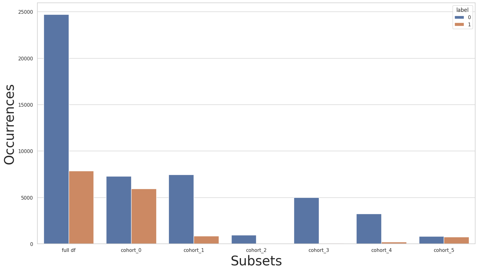
We can now look at the label distribution over each of the relationship cohorts using the plot_value_counts_cohort function, this will be useful to look for data imbalance (with the help of the CohortManager class):

cohort_set = CohortManager(
    cohort_col=["relationship"]
)
cohort_set.fit(X=X_train, y=y_train)
subsets = cohort_set.get_subsets(X_train, y_train, apply_transform=False)

print(y_train.value_counts())
for key in subsets.keys():
    print(f"\n{key}:\n{subsets[key]['y'].value_counts()}\n***********")

plot_value_counts_cohort(y_train, subsets, normalize=False)

0    24720
1     7841
Name: income, dtype: int64

cohort_0:
0    7275
1    5918
Name: income, dtype: int64
***********

cohort_1:
0    7449
1     856
Name: income, dtype: int64
***********

cohort_2:
0    944
1     37
Name: income, dtype: int64
***********

cohort_3:
0    5001
1      67
Name: income, dtype: int64
***********

cohort_4:
0    3228
1     218
Name: income, dtype: int64
***********

cohort_5:
0    823
1    745
Name: income, dtype: int64
***********

Rebalancing the entire dataset

Let’s start by using a simple rebalance strategy using the Rebalance class over the entire dataset. We then plot the new label distributions:

rebalance = dp.Rebalance(verbose=False)
new_X_train, new_y_train = rebalance.fit_resample(X_train, y_train)

cohort_set.fit(X=new_X_train, y=new_y_train)
subsets = cohort_set.get_subsets(new_X_train, new_y_train, apply_transform=False)

print(new_y_train.value_counts())
for key in subsets.keys():
    print(f"\n{key}:\n{subsets[key]['y'].value_counts()}\n***********")

plot_value_counts_cohort(new_y_train, subsets, normalize=False)

0    24720
1    24720
Name: income, dtype: int64

cohort_0:
1    21603
0     7275
Name: income, dtype: int64
***********

cohort_1:
0    7449
1    1423
Name: income, dtype: int64
***********

cohort_2:
0    944
1     40
Name: income, dtype: int64
***********

cohort_3:
0    5001
1      77
Name: income, dtype: int64
***********

cohort_4:
0    3228
1     238
Name: income, dtype: int64
***********

cohort_5:
1    1339
0     823
Name: income, dtype: int64
***********

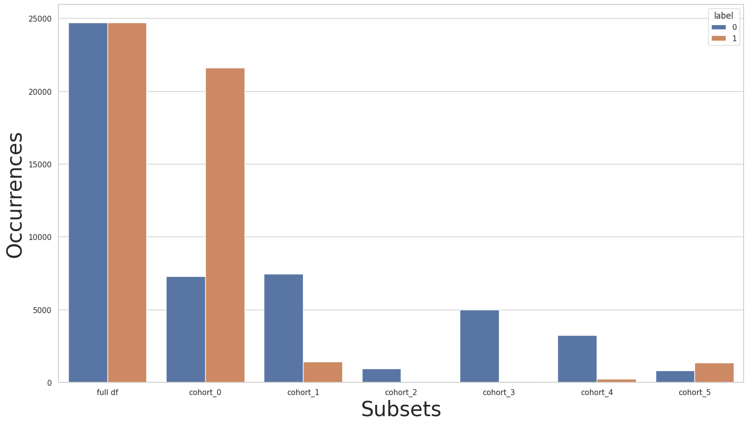
Notice that the label distribution became imbalanced towards the opposite class in cohort_0 after rebalancing. Let’s now use the baseline pipeline with the rebalanced dataset, check the results for the relationship cohorts, and compare it to Baseline 3:

#EXPERIMENT: Baseline 4

pipe = Pipeline([
            ("scaler", dp.DataStandardScaler(verbose=False)),
            ("encoder", dp.EncoderOHE(verbose=False)),
            ("estimator", get_model()),
        ])
pipe.fit(new_X_train, new_y_train)
pred_org = pipe.predict_proba(X_test)

pred_train_org = pipe.predict_proba(new_X_train)
metrics_train, th_dict = fetch_cohort_results(new_X_train, new_y_train, pred_train_org, cohort_col=["relationship"], return_th_dict=True)
fetch_cohort_results(X_test, y_test, pred_org, cohort_col=["relationship"], fixed_th=th_dict)

	cohort	cht_query	roc	precision	recall	f1	accuracy	threshold	cht_size
0	all	all	0.921874	0.804539	0.819558	0.811534	0.860574	0.516163	16281
1	cohort_0	(`relationship` == " Husband")	0.835034	0.758721	0.727895	0.729487	0.743830	0.744579	6523
2	cohort_1	(`relationship` == " Not-in-family")	0.899895	0.696652	0.812623	0.733305	0.876344	0.162488	4278
3	cohort_2	(`relationship` == " Other-relative")	0.953791	0.636910	0.839216	0.687639	0.939048	0.099639	525
4	cohort_3	(`relationship` == " Own-child")	0.932081	0.551532	0.866812	0.558926	0.869877	0.015063	2513
5	cohort_4	(`relationship` == " Unmarried")	0.903355	0.617015	0.792140	0.650214	0.871352	0.089455	1679
6	cohort_5	(`relationship` == " Wife")	0.861501	0.782736	0.780328	0.781221	0.783748	0.603711	763

As expected, we didn’t have a considerable improvement. The only meaningful improvement is for cohort_2. For the other cohorts, we either got a slight increase or decrease in some metrics (compared to Baseline 3).

We’ll now try using the cohort-based pipeline over the rebalanced dataset:

#EXPERIMENT: Cohort 4

cht_manager = CohortManager(
    transform_pipe=[
        dp.DataStandardScaler(verbose=False),
        dp.EncoderOHE(drop=False, unknown_err=False, verbose=False),
        get_model()
    ],
    cohort_col=["relationship"]
)
cht_manager.fit(new_X_train, new_y_train)
pred_cht = cht_manager.predict_proba(X_test)

pred_train = cht_manager.predict_proba(new_X_train)
metrics_train, th_dict = fetch_cohort_results(new_X_train, new_y_train, pred_train, cohort_col=["relationship"], return_th_dict=True)
fetch_cohort_results(X_test, y_test, pred_cht, cohort_col=["relationship"], fixed_th=th_dict)

	cohort	cht_query	roc	precision	recall	f1	accuracy	threshold	cht_size
0	all	all	0.917939	0.807377	0.802695	0.804988	0.860328	0.558872	16281
1	cohort_0	(`relationship` == " Husband")	0.831617	0.756983	0.728497	0.730241	0.743830	0.735383	6523
2	cohort_1	(`relationship` == " Not-in-family")	0.900655	0.712755	0.789351	0.742101	0.891772	0.189098	4278
3	cohort_2	(`relationship` == " Other-relative")	0.905359	0.986641	0.533333	0.555730	0.973333	0.972915	525
4	cohort_3	(`relationship` == " Own-child")	0.918816	0.993800	0.647727	0.724951	0.987664	0.889831	2513
5	cohort_4	(`relationship` == " Unmarried")	0.881868	0.690658	0.721922	0.704817	0.934485	0.234289	1679
6	cohort_5	(`relationship` == " Wife")	0.835875	0.758354	0.759105	0.758665	0.760157	0.577520	763

The results shown above depict a similar scenario to the previous results (baseline pipeline over the rebalanced dataset): an improvement over some cohorts and performance reduction for other cohorts. Once again, this is because a different number of data points were added to each cohort, due to the nature of the SMOTE rebalancing technique (used in the Rebalance class).

Rebalancing only a few cohorts

Let’s try to mitigate these issues by rebalancing only a few cohorts because as we’ve seen in the label distribution of the original dataset, only a few cohorts have a serious label imbalance. This way, we’ll try to improve the results of only a few cohorts. In the following cell, we use the Rebalance class together with the CohortManager in order to rebalance only cohorts cohort_2 and cohort_3:

c0_pipe = []
c1_pipe = []
c2_pipe = [dp.Rebalance(strategy_over=0.2, verbose=False)]
c3_pipe = [dp.Rebalance(strategy_over=0.2, verbose=False)]
c4_pipe = []
c5_pipe = []

rebalance_cohort = CohortManager(
    transform_pipe=[c0_pipe, c1_pipe, c2_pipe, c3_pipe, c4_pipe, c5_pipe],
    cohort_col=["relationship"]
)
new_X_train, new_y_train = rebalance_cohort.fit_resample(X_train, y_train)

subsets = rebalance_cohort.get_subsets(new_X_train, new_y_train, apply_transform=False)

plot_value_counts_cohort(new_y_train, subsets, normalize=False)

We’ll now repeat the same experiments as before. We’ll first train the baseline pipeline over the new rebalanced dataset:

#EXPERIMENT: Baseline 5

pipe = Pipeline([
            ("scaler", dp.DataStandardScaler(verbose=False)),
            ("encoder", dp.EncoderOHE(verbose=False)),
            ("estimator", get_model()),
        ])
pipe.fit(new_X_train, new_y_train)
pred_org = pipe.predict_proba(X_test)

pred_train_org = pipe.predict_proba(new_X_train)
metrics_train, th_dict = fetch_cohort_results(new_X_train, new_y_train, pred_train_org, cohort_col=["relationship"], return_th_dict=True)
fetch_cohort_results(X_test, y_test, pred_org, cohort_col=["relationship"], fixed_th=th_dict)

	cohort	cht_query	roc	precision	recall	f1	accuracy	threshold	cht_size
0	all	all	0.922955	0.766924	0.838044	0.785133	0.821325	0.248997	16281
1	cohort_0	(`relationship` == " Husband")	0.849175	0.753510	0.755060	0.754039	0.755787	0.426605	6523
2	cohort_1	(`relationship` == " Not-in-family")	0.900467	0.673765	0.810531	0.708795	0.853436	0.160477	4278
3	cohort_2	(`relationship` == " Other-relative")	0.949020	0.603624	0.827451	0.644309	0.916190	0.183510	525
4	cohort_3	(`relationship` == " Own-child")	0.920128	0.584059	0.781099	0.621451	0.942698	0.211052	2513
5	cohort_4	(`relationship` == " Unmarried")	0.905372	0.628509	0.794202	0.665738	0.885051	0.096555	1679
6	cohort_5	(`relationship` == " Wife")	0.870593	0.775162	0.776953	0.773108	0.773263	0.447575	763

Once again, we did get improvements for some cohorts, and performance reduction for others. Let’s try using the cohort-based pipeline over this new rebalanced dataset:

#EXPERIMENT: Cohort 5

cht_manager = CohortManager(
    transform_pipe=[
        dp.DataStandardScaler(verbose=False),
        dp.EncoderOHE(drop=False, unknown_err=False, verbose=False),
        get_model()
    ],
    cohort_col=["relationship"]
)
cht_manager.fit(new_X_train, new_y_train)
pred_cht = cht_manager.predict_proba(X_test)

pred_train = cht_manager.predict_proba(new_X_train)
metrics_train, th_dict = fetch_cohort_results(new_X_train, new_y_train, pred_train, cohort_col=["relationship"], return_th_dict=True)
fetch_cohort_results(X_test, y_test, pred_cht, cohort_col=["relationship"], fixed_th=th_dict)

	cohort	cht_query	roc	precision	recall	f1	accuracy	threshold	cht_size
0	all	all	0.921497	0.781029	0.836569	0.799910	0.840059	0.268842	16281
1	cohort_0	(`relationship` == " Husband")	0.847310	0.763712	0.760496	0.761651	0.765445	0.467993	6523
2	cohort_1	(`relationship` == " Not-in-family")	0.894365	0.705684	0.785957	0.735656	0.887564	0.162837	4278
3	cohort_2	(`relationship` == " Other-relative")	0.888235	0.863484	0.599020	0.651590	0.975238	0.937766	525
4	cohort_3	(`relationship` == " Own-child")	0.902776	0.780872	0.724235	0.749223	0.984481	0.470157	2513
5	cohort_4	(`relationship` == " Unmarried")	0.872706	0.707712	0.739665	0.722286	0.938654	0.209798	1679
6	cohort_5	(`relationship` == " Wife")	0.830681	0.734595	0.735099	0.734815	0.736566	0.510850	763

Let’s compare this last results with the results obtained by using the cohort-base pipeline over the original dataset (Cohort 3): by using the rebalanced dataset, we managed to improve the performance for cohort_2 and cohort_3, where the performance increase for cohort_2 was considerably higher.