Using Pipelines

The dataprocessing library works with the Pipeline class from SKLearn. In this notebook, we show a few examples of how to use pipelines with transformers from the dataprocessing library.

from typing import Union

import pandas as pd
import numpy as np
from sklearn.svm import SVC
from sklearn.cluster import KMeans
from sklearn.preprocessing import StandardScaler
from sklearn.impute import SimpleImputer
from sklearn.pipeline import Pipeline
import uci_dataset as database

from raimitigations.utils import evaluate_set, split_data
import raimitigations.dataprocessing as dp

In this notebook, we’ll use the thyroid disease dataset. Let’s load this dataset and take a look at it:

df = database.load_thyroid_disease()
label_col = "sick-euthyroid"
df[label_col] = df[label_col].replace({"sick-euthyroid": 1, "negative": 0})
df

	sick-euthyroid	age	sex	on_thyroxine	query_on_thyroxine	on_antithyroid_medication	thyroid_surgery	query_hypothyroid	query_hyperthyroid	pregnant	...	T3_measured	T3	TT4_measured	TT4	T4U_measured	T4U	FTI_measured	FTI	TBG_measured	TBG
0	1	72.0	M	f	f	f	f	f	f	f	...	y	1.0	y	83.0	y	0.95	y	87.0	n	NaN
1	1	45.0	F	f	f	f	f	f	f	f	...	y	1.0	y	82.0	y	0.73	y	112.0	n	NaN
2	1	64.0	F	f	f	f	f	f	f	f	...	y	1.0	y	101.0	y	0.82	y	123.0	n	NaN
3	1	56.0	M	f	f	f	f	f	f	f	...	y	0.8	y	76.0	y	0.77	y	99.0	n	NaN
4	1	78.0	F	t	f	f	f	t	f	f	...	y	0.3	y	87.0	y	0.95	y	91.0	n	NaN
...	...	...	...	...	...	...	...	...	...	...	...	...	...	...	...	...	...	...	...	...	...
3158	0	40.0	F	f	f	f	f	f	f	f	...	y	1.2	y	76.0	y	0.90	y	84.0	n	NaN
3159	0	69.0	F	f	f	f	f	f	f	f	...	y	1.8	y	126.0	y	1.02	y	124.0	n	NaN
3160	0	58.0	F	f	f	f	f	f	f	f	...	y	1.7	y	86.0	y	0.91	y	95.0	n	NaN
3161	0	29.0	F	f	f	f	f	f	f	f	...	y	1.8	y	99.0	y	1.01	y	98.0	n	NaN
3162	0	56.0	F	t	f	f	f	f	f	f	...	y	1.8	y	139.0	y	0.97	y	143.0	n	NaN

3163 rows × 26 columns

df.info()

<class 'pandas.core.frame.DataFrame'>
RangeIndex: 3163 entries, 0 to 3162
Data columns (total 26 columns):
 #   Column                     Non-Null Count  Dtype
---  ------                     --------------  -----
 0   sick-euthyroid             3163 non-null   int64
 1   age                        2717 non-null   float64
 2   sex                        3090 non-null   object
 3   on_thyroxine               3163 non-null   object
 4   query_on_thyroxine         3163 non-null   object
 5   on_antithyroid_medication  3163 non-null   object
 6   thyroid_surgery            3163 non-null   object
 7   query_hypothyroid          3163 non-null   object
 8   query_hyperthyroid         3163 non-null   object
 9   pregnant                   3163 non-null   object
 10  sick                       3163 non-null   object
 11  tumor                      3163 non-null   object
 12  lithium                    3163 non-null   object
 13  goitre                     3163 non-null   object
 14  TSH_measured               3163 non-null   object
 15  TSH                        2695 non-null   float64
 16  T3_measured                3163 non-null   object
 17  T3                         2468 non-null   float64
 18  TT4_measured               3163 non-null   object
 19  TT4                        2914 non-null   float64
 20  T4U_measured               3163 non-null   object
 21  T4U                        2915 non-null   float64
 22  FTI_measured               3163 non-null   object
 23  FTI                        2916 non-null   float64
 24  TBG_measured               3163 non-null   object
 25  TBG                        260 non-null    float64
dtypes: float64(7), int64(1), object(18)
memory usage: 642.6+ KB

Comparing different pipelines

Using pipelines allow us to compare different pre-processing methods in a easy and efficient way. Here we will build different pipelines, each with different transformations, and then compare the results obtained for each one. But before we can do this, let’s build a function that calls the pipeline’s fit and predict_proba methods, followed by the computation of a few metrics, such as ROC AUC, F1, precision, recall, accuracy, and the confusion matrix. To compute these metrics, we use the evaluate_set function from the utils.model_utils module.

def fit_and_get_results_bin(
    pipeline: Pipeline,
    x_train: pd.DataFrame,
    y_train: pd.DataFrame,
    x_test: pd.DataFrame,
    y_test: pd.DataFrame,
    best_th_auc: bool=True
):
    pipeline.fit(x_train, y_train)
    pred_test = pipeline.predict_proba(x_test)
    _ = evaluate_set(y_test, pred_test, regression=False, plot_pr=False, best_th_auc=best_th_auc, classes=pipeline.classes_)

We’ll also test the efficiency of using scalers over the numerical features of the dataset. It only makes sense to scale the numerical features that doesn’t represent one-hot encodings, so let’s get the list of all float columns from the dataset. This list will represent the list of columns to which we’ll apply the scaler transformations.

float_cols = [col for col in df.columns if 'float' in df[col].dtype.name]
float_cols

['age', 'TSH', 'T3', 'TT4', 'T4U', 'FTI', 'TBG']

Each pipeline can have different transformations. However, some of these transformations could be repeated among different pipelines. For example, all pipelines should have an imputer transformer. In the following cell we’ll instantiate a few transformers in an effort to simplify the pipeline creation process.

ohe_encoder = dp.EncoderOHE(drop=False, unknown_err=False, verbose=False)
imputer = dp.BasicImputer(numerical={'missing_values':np.nan,
                                                                    'strategy':'constant',
                                                                    'fill_value':-1},
                          verbose=False)
feat_sel = dp.CatBoostSelection(catboost_log=False, verbose=False)
cor_feat = dp.CorrelatedFeatures(save_json=False)

Now we just have to split the original dataset into train and test sets. After that, we can start comparing the different pipelines.

train_x, test_x, train_y, test_y = split_data(df, label_col, test_size=0.2)

Pipeline 0

pipe0 = Pipeline([
            ("encoder", ohe_encoder),
            ("imputer", imputer),
            ("estimator", SVC(probability=True)),
        ])
fit_and_get_results_bin(pipe0, train_x, train_y, test_x, test_y, best_th_auc=True)

[[501  73]
 [  7  52]]

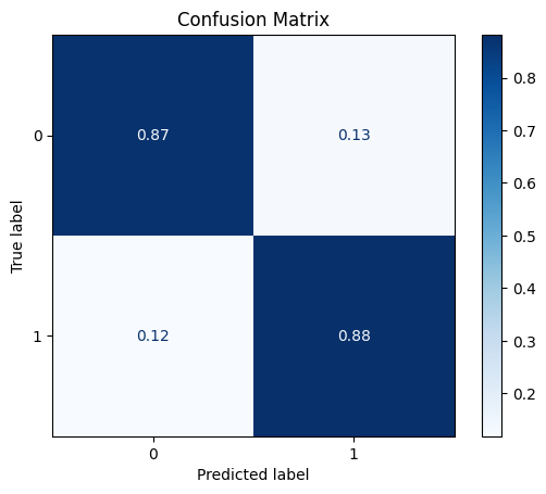
ROC AUC: 0.9299001948857261
Precision: 0.7011102362204724
Recall: 0.877089115927479
F1: 0.7456401189423771
Accuracy: 0.8736176935229067
Optimal Threshold (ROC curve): 0.1250311491470217
Optimal Threshold (Precision x Recall curve): 0.251147863435757
Threshold used: 0.1250311491470217

Pipeline 1

pipe1 = Pipeline([
            ("encoder", ohe_encoder),
            ("imputer", imputer),
            ("scaler", dp.DataStandardScaler(include_cols=float_cols, verbose=False)),
            ("estimator", SVC(probability=True)),
        ])
fit_and_get_results_bin(pipe1, train_x, train_y, test_x, test_y, best_th_auc=True)

[[555  19]
 [  7  52]]

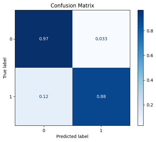
ROC AUC: 0.9250280517333019
Precision: 0.8599694250914741
Recall: 0.9241274434536113
F1: 0.888556338028169
Accuracy: 0.9589257503949447
Optimal Threshold (ROC curve): 0.29745720239980394
Optimal Threshold (Precision x Recall curve): 0.43828324901046595
Threshold used: 0.29745720239980394

Pipeline 2

pipe2 = Pipeline([
            ("encoder", ohe_encoder),
            ("imputer", imputer),
            ("scaler", dp.DataStandardScaler(include_cols=float_cols)),
            ("feat_sel", feat_sel),
            ("estimator", SVC(probability=True)),
        ])
fit_and_get_results_bin(pipe2, train_x, train_y, test_x, test_y, best_th_auc=True)

/home/matheus/miniconda3/envs/rai/lib/python3.9/site-packages/catboost/core.py:1222: FutureWarning: iteritems is deprecated and will be removed in a future version. Use .items instead.
  self._init_pool(data, label, cat_features, text_features, embedding_features, pairs, weight,

[[548  26]
 [  7  52]]

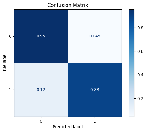
ROC AUC: 0.9340046063898896
Precision: 0.827027027027027
Recall: 0.9180298824780015
F1: 0.8649473405183838
Accuracy: 0.9478672985781991
Optimal Threshold (ROC curve): 0.22808377020466744
Optimal Threshold (Precision x Recall curve): 0.4029785100782772
Threshold used: 0.22808377020466744

Using SKLearn and Dataprocessing transformers in the same Pipeline

The transformations in SKLearn always return a numpy array, while the transformers in our dataprocessing library usually operate over a Pandas DataFrame (although these transformers also accept numpy arrays as input). The latter uses dataframes in order to allow it to filter specific columns, just like we did when we created the DataStandardScaler object and specified that only the columns in the float_cols list should be scaled. With a numpy array, we can also do this, but instead of using column names, we are forced to use the column indices instead, since numpy arrays doesn’t have column names.

In this scenario, when we place a transformer from the SKLearn library before a transformer from the dataprocessing library in a Pipeline, we must be aware that we’ll lose the column names (considering that the input to the Pipeline is indeed a Pandas dataframe) after the sklearn transformer calls its transform() method. This way, all of the transformers after this point will have to use column indices instead of column names, as depicted in the following example. In this example, we’ll use the SKLearn’s SimpleImputer instead of using our similar class, the BasicImputer, just so we can test the behavior of the Pipeline class with transformers from both SKLearn and dataprocessing libraries. We’ll execute the following steps in this pipeline:

1. encode the columns “sex” and “on_thyroxine” using one-hot encoding,

2. impute missing data by replacing it with a -100 value,

3. apply a min-max scaler over the column “age”,

4. apply an ordinal encoding over all of the remaining categorical variables.

pipe = Pipeline([
            ("encoder_ohe", dp.EncoderOHE(col_encode=["sex", "on_thyroxine"])), # dataprocessing
            ("imputer", SimpleImputer(strategy="constant", fill_value=-100)),   # sklearn
            ("scaler", dp.DataMinMaxScaler(include_cols=[0])),                  # dataprocessing
            ("ordinal_encoder", dp.EncoderOrdinal(verbose=False)),              # dataprocessing
        ])
pipe.fit(train_x, train_y)
new_x_test = pipe.transform(test_x)
new_x_test

	0	1	2	3	4	5	6	7	8	9	...	16	17	18	19	20	21	22	23	24	25
0	0.641414	0	0	0	0	0	0	0	0	0	...	10.0	1	0.9	1	12.0	0	-100	0	0	0
1	0.929293	0	0	0	0	0	0	0	0	0	...	162.0	1	1.03	1	158.0	0	-100	0	0	0
2	0.000000	0	0	0	0	0	0	0	0	0	...	175.0	1	0.86	1	204.0	0	-100	0	1	0
3	0.858586	0	0	0	1	0	0	0	0	0	...	69.0	1	0.83	1	83.0	0	-100	0	0	0
4	0.808081	0	0	0	0	0	0	0	0	0	...	130.0	1	0.94	1	138.0	0	-100	1	0	0
...	...	...	...	...	...	...	...	...	...	...	...	...	...	...	...	...	...	...	...	...	...
628	0.863636	0	0	0	0	0	0	0	0	0	...	137.0	1	1.11	1	123.0	0	-100	1	0	0
629	0.606061	0	0	0	1	0	0	0	0	0	...	110.0	1	0.92	1	120.0	0	-100	0	0	0
630	0.000000	0	0	0	0	0	0	0	0	0	...	79.0	1	1.0	1	80.0	0	-100	0	0	0
631	0.858586	0	0	0	1	0	0	0	0	0	...	68.0	1	0.0	1	78.0	0	-100	0	0	0
632	0.616162	0	0	0	0	0	0	0	0	0	...	-100	0	-100	0	-100	1	110.0	0	0	0

633 rows × 26 columns

As we can see in the previous cell, we used column names when instantiating the EncoderOHE class, but used column indices when specifying the columns that should be scaled using the DataMinMaxScaler. This is required because the SimpleImputer object returns a numpy array, which has no column names. From there onward, the column names are lost. We could use indices for all transformers. This would result in the same new x test set, as showed in the following cell:

pipe = Pipeline([
            ("encoder_ohe", dp.EncoderOHE(col_encode=[1, 2])),                  # dataprocessing
            ("imputer", SimpleImputer(strategy="constant", fill_value=-100)),   # sklearn
            ("scaler", dp.DataMinMaxScaler(include_cols=[0])),                  # dataprocessing
            ("ordinal_encoder", dp.EncoderOrdinal(verbose=False)),              # dataprocessing
        ])
pipe.fit(train_x, train_y)
new_x_test = pipe.transform(test_x)
new_x_test

	0	1	2	3	4	5	6	7	8	9	...	16	17	18	19	20	21	22	23	24	25
0	0.641414	0	0	0	0	0	0	0	0	0	...	10.0	1	0.9	1	12.0	0	-100	0	0	0
1	0.929293	0	0	0	0	0	0	0	0	0	...	162.0	1	1.03	1	158.0	0	-100	0	0	0
2	0.000000	0	0	0	0	0	0	0	0	0	...	175.0	1	0.86	1	204.0	0	-100	0	1	0
3	0.858586	0	0	0	1	0	0	0	0	0	...	69.0	1	0.83	1	83.0	0	-100	0	0	0
4	0.808081	0	0	0	0	0	0	0	0	0	...	130.0	1	0.94	1	138.0	0	-100	1	0	0
...	...	...	...	...	...	...	...	...	...	...	...	...	...	...	...	...	...	...	...	...	...
628	0.863636	0	0	0	0	0	0	0	0	0	...	137.0	1	1.11	1	123.0	0	-100	1	0	0
629	0.606061	0	0	0	1	0	0	0	0	0	...	110.0	1	0.92	1	120.0	0	-100	0	0	0
630	0.000000	0	0	0	0	0	0	0	0	0	...	79.0	1	1.0	1	80.0	0	-100	0	0	0
631	0.858586	0	0	0	1	0	0	0	0	0	...	68.0	1	0.0	1	78.0	0	-100	0	0	0
632	0.616162	0	0	0	0	0	0	0	0	0	...	-100	0	-100	0	-100	1	110.0	0	0	0

633 rows × 26 columns

Using column indices is not as intuitive as using column names. Using indices is also more error prone, especially when dealing with a pipeline with transformations that could change the order of the columns, such as the EncoderOHE and feature selection methods. In these scenarios, the index of a column might change in the middle of the pipeline, making it harder for the user to know exactly the column index that they should use to apply a specific operation over a specific column. Therefore, it is of interest to the user to continue to use only column names when possible. In the remainder of this section, we’ll present three solutions to this problem.

Solution 1: use the Pipeline class with only transformers from the dataprocessing library

The first solution is pretty straightforward: use only transformers from the dataprocessing library. Note that an estimator from SKLearn or other libraries could still be used in the end of the pipeline, but the transformers used must be always from the dataprocessing library. Since all transformers from this library operate over Pandas Dataframes, and if all transformers in the pipeline return dataframes, then at no point in the pipeline this dataframe will be lost. This guarantees that all transformers will receive a dataframe as input, without losing the column names. As a result, all transformers are allowed to use filters based on column names.

Let’s recreate the previous pipeline using only transformers from our library. For this, we’ll replace the SimpleImputer by the BasicImputer. This allows us to use column names when specifying which columns the DataMinMaxScaler should be applied on:

miss_dict ={'missing_values':np.nan, 'strategy':'constant', 'fill_value':-100}

pipe = Pipeline([
            ("encoder_ohe", dp.EncoderOHE(col_encode=["sex", "on_thyroxine"])),                         # dataprocessing
            ("imputer", dp.BasicImputer(numerical=miss_dict, categorical=miss_dict, verbose=False)),    # dataprocessing
            ("scaler", dp.DataMinMaxScaler(include_cols=["age"])),                                      # dataprocessing
            ("ordinal_encoder", dp.EncoderOrdinal(verbose=False)),                                      # dataprocessing
        ])
pipe.fit(train_x, train_y)
new_x_test = pipe.transform(test_x)
new_x_test

	age	query_on_thyroxine	on_antithyroid_medication	thyroid_surgery	query_hypothyroid	query_hyperthyroid	pregnant	sick	tumor	lithium	...	TT4	T4U_measured	T4U	FTI_measured	FTI	TBG_measured	TBG	sex_M	sex_nan	on_thyroxine_t
3073	0.641414	0	0	0	0	0	0	0	0	0	...	10.0	1	0.90	1	12.0	0	-100.0	0	0	0
1839	0.929293	0	0	0	0	0	0	0	0	0	...	162.0	1	1.03	1	158.0	0	-100.0	0	0	0
3096	0.000000	0	0	0	0	0	0	0	0	0	...	175.0	1	0.86	1	204.0	0	-100.0	0	1	0
1147	0.858586	0	0	0	1	0	0	0	0	0	...	69.0	1	0.83	1	83.0	0	-100.0	0	0	0
2413	0.808081	0	0	0	0	0	0	0	0	0	...	130.0	1	0.94	1	138.0	0	-100.0	1	0	0
...	...	...	...	...	...	...	...	...	...	...	...	...	...	...	...	...	...	...	...	...	...
148	0.863636	0	0	0	0	0	0	0	0	0	...	137.0	1	1.11	1	123.0	0	-100.0	1	0	0
2526	0.606061	0	0	0	1	0	0	0	0	0	...	110.0	1	0.92	1	120.0	0	-100.0	0	0	0
593	0.000000	0	0	0	0	0	0	0	0	0	...	79.0	1	1.00	1	80.0	0	-100.0	0	0	0
2203	0.858586	0	0	0	1	0	0	0	0	0	...	68.0	1	0.00	1	78.0	0	-100.0	0	0	0
1302	0.616162	0	0	0	0	0	0	0	0	0	...	-100.0	0	-100.00	0	-100.0	1	110.0	0	0	0

633 rows × 26 columns

Solution 2: use the SklearnTransformerWrapper class

If there is a specific transformer from the SKLearn library not present in the dataprocessing library, then the user has no alternative but to use the SKLearn transformer. The SklearnTransformerWrapper class, from the Feature Engine library, is a wrapper for transformers from the SKLearn library that forces, among other features, forces the output of the transformers to be a pandas dataframe if the input is also a dataframe. This solves our problem, since this way the dataframe is never lost. To do this, the user must pass the transformer object to the SklearnTransformerWrapper constructor when instantiating it. The SklearnTransformerWrapper object will then allow users to use the fit and transform methods, but now, the transform method returns a pandas dataframe instead of a numpy array.

The following cell shows how to use the SklearnTransformerWrapper to wrap a transformer from the SKLearn library and then use it in a Pipeline. Before running the following cell, make sure to install the feature-engine package following this link.

from feature_engine.wrappers import SklearnTransformerWrapper

imputer = SklearnTransformerWrapper(transformer=SimpleImputer(strategy="constant", fill_value=-100))

pipe = Pipeline([
            ("encoder_ohe", dp.EncoderOHE(col_encode=["sex", "on_thyroxine"])), # dataprocessing
            ("imputer", imputer),                                               # sklearn
            ("scaler", dp.DataMinMaxScaler(include_cols=["age"])),                  # dataprocessing
            ("ordinal_encoder", dp.EncoderOrdinal(verbose=False)),              # dataprocessing
        ])
pipe.fit(train_x, train_y)
new_x_test = pipe.transform(test_x)
new_x_test

	age	query_on_thyroxine	on_antithyroid_medication	thyroid_surgery	query_hypothyroid	query_hyperthyroid	pregnant	sick	tumor	lithium	...	TT4	T4U_measured	T4U	FTI_measured	FTI	TBG_measured	TBG	sex_M	sex_nan	on_thyroxine_t
3073	0.641414	0	0	0	0	0	0	0	0	0	...	10.0	1	0.9	1	12.0	0	-100	0	0	0
1839	0.929293	0	0	0	0	0	0	0	0	0	...	162.0	1	1.03	1	158.0	0	-100	0	0	0
3096	0.000000	0	0	0	0	0	0	0	0	0	...	175.0	1	0.86	1	204.0	0	-100	0	1	0
1147	0.858586	0	0	0	1	0	0	0	0	0	...	69.0	1	0.83	1	83.0	0	-100	0	0	0
2413	0.808081	0	0	0	0	0	0	0	0	0	...	130.0	1	0.94	1	138.0	0	-100	1	0	0
...	...	...	...	...	...	...	...	...	...	...	...	...	...	...	...	...	...	...	...	...	...
148	0.863636	0	0	0	0	0	0	0	0	0	...	137.0	1	1.11	1	123.0	0	-100	1	0	0
2526	0.606061	0	0	0	1	0	0	0	0	0	...	110.0	1	0.92	1	120.0	0	-100	0	0	0
593	0.000000	0	0	0	0	0	0	0	0	0	...	79.0	1	1.0	1	80.0	0	-100	0	0	0
2203	0.858586	0	0	0	1	0	0	0	0	0	...	68.0	1	0.0	1	78.0	0	-100	0	0	0
1302	0.616162	0	0	0	0	0	0	0	0	0	...	-100	0	-100	0	-100	1	110.0	0	0	0

633 rows × 26 columns

Solution 3: Wrap the Pipeline class and apply solution 2 automatically

We can also create a wrapper over the Pipeline class that automatically applies Solution 2 to the transformers in the pipeline. This extension, called here the PipelineWrapper, provides a simple modification: all transformers that are not from the dataprocessing library are wrapped around the SklearnTransformerWrapper class. Therefore, the PipelineWrapper executes the previous solution internally, removing the burden of wrapping all of SKLearn’s transformers from the hands of the user. The PipelineWrapper doesn’t change any other behavior from the Pipeline class, and therefore, the latter can be replaced by the former without any changes in the behavior of the code.

First, let’s create the PipelineWrapper class. This class inherits from the Pipeline class. The only modification that we make is that we call a new method, called **_wrap_skl_transf(), in the init method. This method will check all transformers in the pipeline and wrap all of the SKLearn’s transformers in theSklearnTransformerWrapper**. This guarantees that, if the input is a pandas dataframe, the transformers from SKLearn will also output a dataframe.

from feature_engine.wrappers.wrappers import _ALL_TRANSFORMERS

class PipelineWrapper(Pipeline):

    # -----------------------------------
    def __init__(self, steps, *, memory=None, verbose=False):
        super().__init__(steps, memory=memory, verbose=verbose)
        self._wrap_skl_transf()

    # -----------------------------------
    def _wrap_skl_transf(self):
        for i in range(len(self.steps)):
            name, transform = self.steps[i]
            if not isinstance(transform, dp.DataProcessing):
                if not isinstance(transform, SklearnTransformerWrapper):
                    if transform.__class__.__name__ in _ALL_TRANSFORMERS:
                        transform = SklearnTransformerWrapper(transformer=transform)
                        self.steps[i] = (name, transform)

Now let’s use the PipelineWrapper instead of the Pipeline class. Note that nothing changes, except that now we can use the column names even after a transformer from the SKLearn library.

pipe = PipelineWrapper([
            ("encoder_ohe", dp.EncoderOHE(col_encode=["sex", "on_thyroxine"])), # dataprocessing
            ("imputer", SimpleImputer(strategy="constant", fill_value=-100)),   # sklearn
            ("scaler", dp.DataMinMaxScaler(include_cols=["age"])),              # dataprocessing
            ("ordinal_encoder", dp.EncoderOrdinal(verbose=False)),              # dataprocessing
        ])
pipe.fit(train_x, train_y)
new_x_test = pipe.transform(test_x)
new_x_test

	age	query_on_thyroxine	on_antithyroid_medication	thyroid_surgery	query_hypothyroid	query_hyperthyroid	pregnant	sick	tumor	lithium	...	TT4	T4U_measured	T4U	FTI_measured	FTI	TBG_measured	TBG	sex_M	sex_nan	on_thyroxine_t
3073	0.641414	0	0	0	0	0	0	0	0	0	...	10.0	1	0.9	1	12.0	0	-100	0	0	0
1839	0.929293	0	0	0	0	0	0	0	0	0	...	162.0	1	1.03	1	158.0	0	-100	0	0	0
3096	0.000000	0	0	0	0	0	0	0	0	0	...	175.0	1	0.86	1	204.0	0	-100	0	1	0
1147	0.858586	0	0	0	1	0	0	0	0	0	...	69.0	1	0.83	1	83.0	0	-100	0	0	0
2413	0.808081	0	0	0	0	0	0	0	0	0	...	130.0	1	0.94	1	138.0	0	-100	1	0	0
...	...	...	...	...	...	...	...	...	...	...	...	...	...	...	...	...	...	...	...	...	...
148	0.863636	0	0	0	0	0	0	0	0	0	...	137.0	1	1.11	1	123.0	0	-100	1	0	0
2526	0.606061	0	0	0	1	0	0	0	0	0	...	110.0	1	0.92	1	120.0	0	-100	0	0	0
593	0.000000	0	0	0	0	0	0	0	0	0	...	79.0	1	1.0	1	80.0	0	-100	0	0	0
2203	0.858586	0	0	0	1	0	0	0	0	0	...	68.0	1	0.0	1	78.0	0	-100	0	0	0
1302	0.616162	0	0	0	0	0	0	0	0	0	...	-100	0	-100	0	-100	1	110.0	0	0	0

633 rows × 26 columns