Typical Workflow
This solution package shows how to use a prediction model to increase the response rate to a campaign by recommending how to contact (for example, Email, SMS, or Cold Call) as well as when to contact (day of week and time of day) each lead identified for use in a new campaign.
To demonstrate a typical workflow, we’ll introduce you to a few personas. You can follow along by performing the same steps for each persona.
If you want to follow along and have *not* run the PowerShell script, you must to first create a database table in your SQL Server. You will then need to replace the connection_string at the top of each R file with your database and login information.
Step 1: Server Setup and Configuration with Danny the DB Analyst Ivan the IT Administrator
Campaign database. You can see an example of creating a user in the **Campaign/Resources/exampleuser.sql** query.
This step has already been done on your VM if you deployed it using the 'Deploy to Azure' button.
You can perform these steps in your environment by using the instructions to Setup your On-Prem SQL Server.
The cluster has been created and data loaded for you when you used the Deploy to Azure button on the Quick Start page. Once you complete the walkthrough, you will want to delete this cluster as it incurs expense whether it is in use or not - see HDInsight Cluster Maintenance for more details.
Step 2: Data Prep and Modeling with Debra the Data Scientist
Now let’s meet Debra, the Data Scientist. Debra’s job is to use historical data to predict a model for future campaigns. Debra’s preferred language for developing the models is using R and SQL. She uses Microsoft ML Services with SQL Server 2017 as it provides the capability to run large datasets and also is not constrained by memory restrictions of Open Source R.Debra will develop these models using HDInsight, the managed cloud Hadoop solution with integration to Microsoft ML Server.
After analyzing the data she opted to create multiple models and choose the best one. She will create two machine learning models and compare them, then use the one she likes best to compute a prediction for each combination of day, time, and channel for each lead, and then select the combination with the highest probability of conversion - this will be the recommendation for that lead.
http://CLUSTERNAME.azurehdinsight.net/rstudio.
CampaignOptimization:
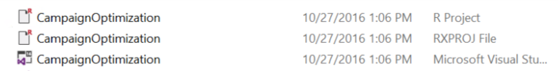
- If you use Visual Studio, double click on the Visual Studio SLN file (the third one in the image above).
- If you use RStudio, double click on the "R Project" file (the first one in the image above)
Now you’re ready to follow along with Debra as she creates the scripts needed for this solution. If you are using Visual Studio, you will see these file in the Solution Explorer tab on the right. In RStudio, the files can be found in the Files tab, also on the right.
-
campaign_main.R is used to define the data and directories and then run all of the steps to process data, perform feature engineering, training, and scoring.
The default input for this script uses 100,000 leads for training models, and will split this into train and test data. After running this script you will see data files in the /Campaign/dev/temp directory on your storage account. Models are stored in the /Campaign/dev/model directory on your storage account. The Hive table
recommendationscontains the 100,000 records with recommendations (recommended_day,recommended_timeandrecommended_channel) created from the best model. - Copy_Dev2Prod.R copies the model information from the dev folder to the prod folder to be used for production. This script must be executed once after campaign_main.R completes, before running campaign_scoring.R. It can then be used again as desired to update the production model. After running this script models created during campaign_main.R are copied into the /var/RevoShare/sshuser/Campaign/prod/model directory.
-
campaign_scoring.R uses the previously trained model and invokes the steps to process data, perform feature engineering and scoring. Use this script after first executing campaign_main.R and Copy_Dev2Prod.R.
The input to this script defaults to 30,000 leads to be scored with the model in the prod directory. After running this script the Hive table
recommendationsnow contains the recommended values for these 30,000 leads.
Below is a summary of the individual steps used for this solution.
- SQLR_connection.R: configures the compute context used in all the rest of the scripts. The connection string is pre-poplulated with the a connection based on your windows credentials.
If you wish to instead use SQL Authentication, use
UID=username;PWD=passwordin place ofTrusted_Connection=Yes. If you wish to the Azure VM from a different machine, modify the connection string to useUID=username;PWD=passwordin place ofTrusted_Connection=Yes. The server name can be found in the Azure Portal under the "Network interfaces" section - use the Public IP Address as the server name. (Make sure not to add spaces between the "=" in the connection string.) - The first few steps prepare the data for training.
- step0_data_generation.R: This file was used to generate data for the current solution - in a real setting it would not be present. It is left here in case you'd like to generate additional data. For now simply ignore this file.
- step1_data_processing.R: Uploads data and performs preprocessing steps -- merging of the input data sets and missing value treatment.
- step2_feature_engineering.R: Performs Feature Engineering and creates the Analytical Dataset. Feature Engineering consists of creating new variables in the cleaned dataset.
SMS_Count,Email_CountandCall_Countare computed: they correspond to the number of times every customer was contacted through these three channels. It also computesPrevious_Channel: for each communication with theLead, it corresponds to theChannelthat was used in the communication that preceded it (a NULL value is attributed to the first record of each Lead). Finally, an aggregation is performed at the Lead Level by keeping the latest record for each one. - After running the step1 and step2 scripts, Debra goes to SQL Server Management Studio to log in and view the results of feature engineering by running the following query:
SELECT TOP 1000 [Lead_Id] ,[Sms_Count] ,[Email_Count] ,[Call_Count] ,[Previous_Channel] FROM [Campaign].[dbo].[CM_AD] - Now she is ready for training the models, using step3_training_evaluation.R. This step will train two different models and evaluate each.
The R script draws the ROC or Receiver Operating Characteristic for each prediction model. It shows the performance of the model in terms of true positive rate and false positive rate, when the decision threshold varies.
</p>
The AUC is a number between 0 and 1. It corresponds to the area under the ROC curve. It is a performance metric related to how good the model is at separating the two classes (converted clients vs. not converted), with a good choice of decision threshold separating between the predicted probabilities. The closer the AUC is to 1, and the better the model is. Given that we are not looking for that optimal decision threshold, the AUC is more representative of the prediction performance than the Accuracy (which depends on the threshold).
Debra will use the AUC to select the champion model to use in the next step.
- Finally step4_campaign_recommendations.R scores data for leads to be used in a new campaign. The code uses the champion model to score each lead multiple times - for each combination of day of week, time of day, and channel - and selects the combination with the highest probability to convert for each lead. This becomes the recommendation for that lead. The scored datatable shows the best way to contact each lead for the next campaign. The recommendations table (
Recommendations) is used for the next campaign the company wants to deploy.This step may take 1-2 minutes to complete. Feel free to skip it if you wish, the data already exists in the SQL database. - After creating the model, Debra runs Copy_Dev2Prod.R to copy the model information from the dev folder to the prod folder, then runs campaign_scoring.R to create recommendations for her new data.
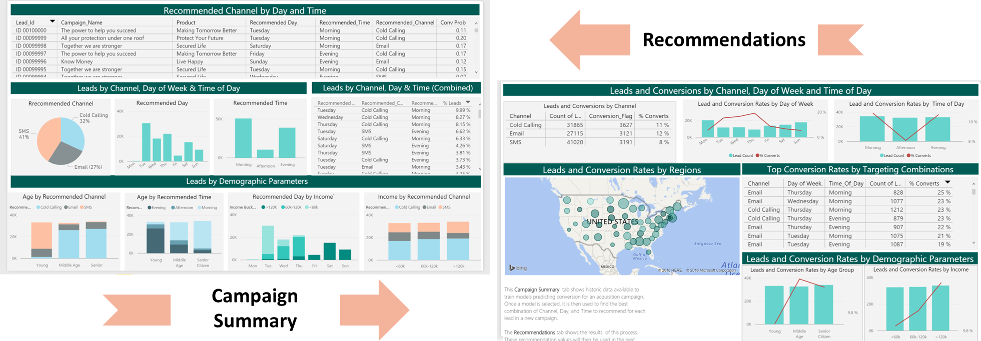
- Once all the above code has been executed, Debra will use PowerBI to visualize the recommendations created from her model.
She uses an ODBC connection to connect to the data, so that it will always show the most recently modeled and scored data.
You can access this dashboard in either of the following ways:
-
Visit the online version.
-
Open the PowerBI file from the Campaign directory on the deployed VM desktop.
-
Install PowerBI Desktop on your computer and download and open the Campaign Optimization Dashboard
-
Install PowerBI Desktop on your computer and download and open the Campaign Optimization HDI Dashboard
 If you want to refresh data in your PowerBI Dashboard, make sure to follow these instructions to setup and use an ODBC connection to the dashboard.
 -
- A summary of this process and all the files involved is described in more detail here.
Step 3: Operationalize with Debra and Danny
Debra has completed her tasks. She has connected to the SQL database, executed code from her R IDE that pushed (in part) execution to the SQL machine to clean the data, create new features, train two models and select the champion model.She has executed code from RStudio that pushed (in part) execution to Hadoop to clean the data, create new features, train two models and select the champion model She has scored data, created recommendations, and also created a summary report which she will hand off to Bernie - see below.
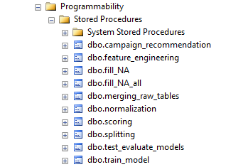
While this task is complete for the current set of leads, our company will want to perform these actions for each new campaign that they deploy. Instead of going back to Debra each time, Danny can operationalize the code in TSQL files which he can then run himself each month for the newest campaign rollouts.
Programmability>Stored Procedures section of the Campaign database.
 You can find this script in the SQLR directory, and execute it yourself by following the PowerShell Instructions.
As noted earlier, this was already executed when your VM was first created. As noted earlier, this is the fastest way to execute all the code included in this solution. (This will re-create the same set of tables and models as the above R scripts.)
You can find this script in the SQLR directory, and execute it yourself by following the PowerShell Instructions.
As noted earlier, this was already executed when your VM was first created. As noted earlier, this is the fastest way to execute all the code included in this solution. (This will re-create the same set of tables and models as the above R scripts.)
Step 4: Deploy and Visualize with Bernie the Business Analyst
Now that the predictions are created and the recommendations have been saved, we will meet our last persona - Bernie, the Business Analyst. Bernie will use the Power BI Dashboard to learn more about the recommendations (second tab). He will also review summaries of the data used to create the model (first tab). While both tabs contain information about Day of Week, Time of Day, and Channel, it is important to understand that on the Recommendations tab this refers to predicted recommendations to use in the future, while on the Summaries tab these values refer to historical data used to create the prediction model that provided the recommendations.
You can access this dashboard in either of the following ways:
-
Visit the online version.
-
Open the PowerBI file from the Campaign directory on the deployed VM desktop.
-
Install PowerBI Desktop on your computer and download and open the Campaign Optimization Dashboard
-
Install PowerBI Desktop on your computer and download and open the Campaign Optimization HDI Dashboard
Bernie will then let the Campaign Team know that they are ready for their next campaign rollout - the data in the Recommendations table contains the recommended time and channel for each lead in the campaign. The team uses these recommendations to contact leads in the new campaign.