Typical Workflow
This solution package shows how to pre-process data (cleaning and feature engineering), train prediction models, and perform scoring on the SQL Server machine. Spark cluster.
To demonstrate a typical workflow, we’ll introduce you to a few personas. You can follow along by performing the same steps for each persona.
If you want to follow along and have not run the PowerShell script, you must to first create a database table in your SQL Server. You will then need to replace the connection_string in the modeling_main.R file with your database and login information.
Step 1: Server Setup and Configuration with Danny the DB Analyst
Let me introduce you to Danny, the Database Analyst. Danny is the main contact for anything regarding the SQL Server database that contains account information, transaction data, and known fraud transactions.
Danny was responsible for installing and configuring the SQL Server. He has added a user with all the necessary permissions to execute R scripts on the server and modify the Fraud_R database. You can see an example of creating a user in the Fraud/Resources/exampleuser.sql.
Step 1: Server Setup and Configuration with Ivan the IT Administrator
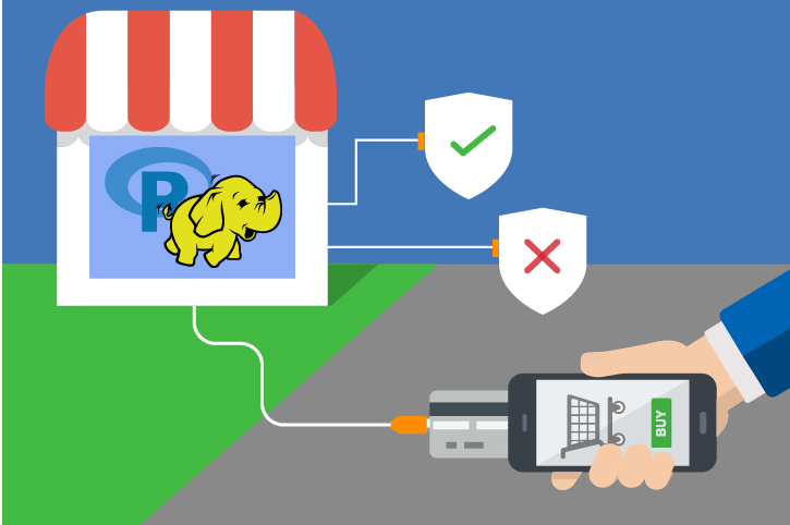
Let me introduce you to Ivan, the IT Administrator. Ivan is responsible for implementation as well as ongoing administration of the Hadoop infrastructure at his company, which uses Hadoop in the Azure Cloud from Microsoft. Ivan created the HDInsight cluster with ML Server for Debra. He also uploaded the data onto the storage account associated with the cluster.
This step has already been done on the VM deployed using the 'Deploy to Azure' button on the Quick Start page.
You can perform these steps in your environment by using the instructions to Setup your On-Prem SQL Server.
The cluster has been created and data loaded for you when you used the 'Deploy to Azure' button on the Quick Start page. Once you complete the walkthrough, you will want to delete this cluster as it incurs expense whether it is in use or not - see HDInsight Cluster Maintenance for more details.
Step 2: Data Prep and Modeling with Debra the Data Scientist
Now let’s meet Debra, the Data Scientist. Debra’s job is to use historical data to predict a model to detect fraud. Debra’s preferred language for developing the models is using R and SQL. She uses Microsoft ML Services with SQL Server 2017 as it provides the capability to run large datasets and also is not constrained by memory restrictions of Open Source R. Debra will develop these models using HDInsight, the managed cloud Hadoop solution with integration to Microsoft ML Server.
http://CLUSTERNAME.azurehdinsight.net/rstudio.
- If you use Visual Studio, double click on the Visual Studio SLN file.
- If you use RStudio, double click on the "R Project" file.
You are ready to follow along with Debra as she creates the model needed for this solution.
If you are using Visual Studio, you will see these file in the Solution Explorer tab on the right. In RStudio, the files can be found in the Files tab, also on the right.
localhost represents a server on the same machine as the R code). If you are connecting to an Azure VM from a different machine, the server name can be found in the Azure Portal under the "Network interfaces" section - use the Public IP Address as the server name.
The steps to create and evaluate the model are described in detail on the For the Data Scientist page. Open and execute the file
modeling_main.R
development_main.R
to run all these steps. You may see some warnings regarding strptime and rxClose. You can ignore these warnings.
After executing this code, you can examine the ROC curve for the Gradient Boosted Tree model in the Plots pane. This gives a transaction level metric on the model.
The metric used for assessing accuracy (performance) depends on how the original cases are processed. If each case is processed on a transaction by transaction basis, you can use a standard performance metric, such as transaction-based ROC curve or AUC.
However, for fraud detection, typically account-level metrics are used, based on the assumption that once a transaction is discovered to be fraudulent (for example, via customer contact), an action will be taken to block all subsequent transactions.
A major difference between account-level metrics and transaction-level metrics is that, typically an account confirmed as a false positive (that is, fraudulent activity was predicted where it did not exist) will not be contacted again during a short period of time, to avoid inconveniencing the customer.
The industry standard fraud detection metrics are ADR vs AFPR and VDR vs AFPR for performance, and transaction level performance, as defined here:
- ADR – Fraud Account Detection Rate. The percentage of detected fraud accounts in all fraud accounts.
- VDR - Value Detection Rate. The percentage of monetary savings, assuming the current fraud transaction triggered a blocking action on subsequent transactions, over all fraud losses.
- AFPR - Account False Positive Ratio. The ratio of detected false positive accounts over detected fraud accounts.
You can see these plots as well in the Plots pane after running modeling_main.R development_main.R .
Step 3: Operationalize with Debra and Danny
Debra has completed her tasks. She has connected to the SQL database, executed code from her R IDE that pushed (in part) execution to the SQL machine to create the fraud model. She has executed code from RStudio that pushed (in part) execution to Hadoop to create the fraud model. She has preprocessed the data, created features, built and evaluated a model. Finally, she created a summary dashboard which she will hand off to Bernie - see below.
Programmability>Stored Procedures section of the Fraud_R database. Find more details about these procedures on the For the Database Analyst page.
Finally, Danny has created a PowerShell script that will re-run the all the steps to train the model.
You can find this script in the SQLR directory, and execute it yourself by following the PowerShell Instructions.
As noted earlier, this was already executed when your VM was first created.
As noted earlier, this is the fastest way to execute all the code included in this solution. (This will re-create the same set of tables and models as the above R scripts.)
Step 4: Deploy and Visualize with Bernie the Business Analyst
Now that the predictions are created we will meet our last persona - Bernie, the Business Analyst. Bernie will use the Power BI Dashboard to examine the data and assess the model prediction using the test data.
You can access this dashboard in any of the following ways:
-
Open the PowerBI file from the Fraud directory on the deployed VM desktop.
-
Install PowerBI Desktop on your computer and download and open the onlinefraud.pbix file.
-
Install PowerBI Desktop on your computer and download and open the onlinefraudHDI.pbix file.
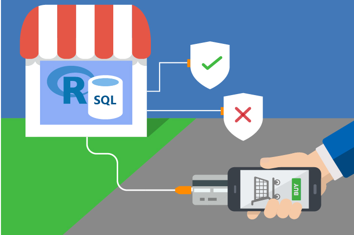
Step 5: Use the Model during Online Transactions
The final goal of this solution is to interrupt a fraudulent transaction before it occurs. Keep in mind that there will be false positives - transctions flagged that are not in fact fraud. For that reason, the decision point when the model returns a high probability of fraud might be to require the purchaser contact a live person to complete the transaction, rather than simply deny the purchase. This solution contains an example of a website that does just that. The example is not meant to be production-quality code, it is meant simply to show how a website might make use of such a model. The example shows the purchase page of a transaction, with the ability to try the same simulated purchase from multiple accounts.
This solution contains an example of a website that does just that. The example is not meant to be production-quality code, it is meant simply to show how a website might make use of such a model. The example shows the purchase page of a transaction, with the ability to try the same simulated purchase from multiple accounts.
To try out this example site, you must first start the lightweight webserver for the site. Open a terminal window or powershell window and type the following command, substituting your own values for the path and username/password:
    cd C:\Solutions\Fraud\Website
    node server.js
You should see the following response:
    Example app listening on port 3000!
    DB Connection Success
Now leave this window open and open the url http://localhost:3000 in your browser.
This site is set up to mimic a sale on a website. “Log in” by selecting an account and then add some items to your shopping cart. Finally, hit the Purchase button to trigger the model scoring. If the model returns a low probability for the transaction, it is not likely to be fraudulent, and the purchase will be accepted. However, if the model returns a high probability, you will see a message that explains the purchaser must contact a support representative to continue.
You can view the model values by opening the Console window on your browser.
- For Edge or Internet Explorer: Press
F12to open Developer Tools, then click on the Console tab. - For FireFox or Chome: Press
Ctrl-Shift-ito open Developer Tools, then click on the Console tab.
Use the Log In button on the site to switch to a different account and try the same transaction again. (Hint: the account number that begins with a “9” is most likely to have a high probability of fraud.)
See more details about this example see For the Web Developer.