Loan Credit Risk

For the Database Analyst - Operationalize with SQL

For businesses that prefers an on-prem solution, the implementation with SQL Server ML Services is a great option, which takes advantage of the power of SQL Server and RevoScaleR (Microsoft ML Server). The implementation with SQL Server ML Services is a great option, which takes advantage of the power of SQL Server and RevoScaleR (Microsoft ML Server).

All the steps can be executed on SQL Server client environment (such as SQL Server Management Studio). We provide a Windows PowerShell script, Loan_Credit_Risk.ps1, which invokes the SQL scripts and demonstrates the end-to-end modeling process.

System Requirements

The following are required to run these scripts:

• SQL server (2016 or higher) with Microsoft ML server (version 9.1.0 or above) installed and configured;
• The SQL user name and password, and the user is configured properly to execute R scripts in-memory;
• SQL Database for which the user has write permission and can execute stored procedures (see create_user.sql);
• Implied authentification is enabled so a connection string can be automatically created in R codes embedded into SQL Stored Procedures (see create_user.sql).
• For more information about SQL server and ML service, please visit: What’s New in SQL Server ML Services

Workflow Automation

Follow the PowerShell instructions to execute all the scripts described below. View the details of all tables created in this solution.

Step 0: Creating Tables

The data sets Loan.csv and Borrower.csv are provided in the Data directory.

In this step, we create two tables, Loan and Borrower in a SQL Server database, and the data is uploaded to these tables using bcp command in PowerShell. This is done through either Load_Data.ps1 or through running the beginning of Loan_Credit_Risk.ps1.

Input:

• Raw data: Loan.csv and Borrower.csv.

Output:

• 2 Tables filled with the raw data: Loan and Borrower (filled through PowerShell).

Related files:

• step0_create_tables.sql

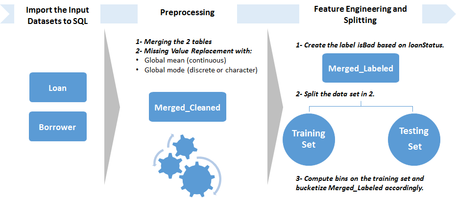
Step 1: Merging and Cleaning

In this step, the two tables are first merged into Merged with an inner join on memberId. This is done through the stored procedure [dbo].[merging].

Then, statistics (mode or mean) of Merged are computed and stored into a table called Stats. This table will be used for the Production pipeline. This is done through the [dbo].[compute_stats] stored procedure.

The raw data is then cleaned. This assumes that the ID variables (loanId and memberId), the date and loanStatus (Variables that will be used to create the label) do not contain blanks. The stored procedure, [fill_NA_mode_mean], will replace the missing values with the mode (categorical variables) or mean (float variables).

Input:

• 2 Tables filled with the raw data: Loan and Borrower (filled through PowerShell).

Output:

• Merged_Cleaned table with the cleaned data.
• Stats table with statistics on the raw data set.

Related files:

• step1_data_preprocessing.sql

Example:

EXEC merging 'Loan' 'Borrower' 'Merged'
EXEC compute_stats 'Merged'
EXEC fill_NA_mode_mean 'Merged' 'Merged_Clean'

Step 2a: Splitting the data set

In this step, we create a stored procedure [dbo].[splitting] that splits the data into a training set and a testing set. It creates a hash function that ensures repeatability and maps loanIds to integers that will be used later to split the data into a training and a testing set.

The splitting is performed prior to feature engineering instead of in the training step because the feature engineering creates bins based on conditional inference trees that should be built only on the training set. If the bins were computed with the whole data set, the evaluation step would be rigged.

Input:

• Merged_Cleaned Table.

Output:

• Hash_Id table containing the loanId and mapping through the hash function.

Related files:

• step2a_splitting.sql

Example:

EXEC splitting 'Merged_Clean'

Step 2b: Feature Engineering

For feature engineering, we want to design new features:

• Categorical versions of all the numeric variables. This is done for interpretability and is a standard practice in the Credit Score industry.
• isBad: the label, specifying whether the loan has been charged off or has defaulted (isBad = 1) or if it is in good standing (isBad = 0), based on loanStatus.

In this step, we first create a stored procedure [dbo].[compute_bins]. It uses the CRAN R package smbinning that builds a conditional inference tree on the training set (to which we append the binary label isBad) in order to get the optimal bins to be used for the numeric variables we want to bucketize. Because some of the numeric variables have too few unique values, or because the binning function did not return significant splits, we decided to manually specify default bins for all the variables in case smbinning failed to provide them. These default bins have been determined through an analysis of the data or through running smbinning on a larger data set. The computed and specified bins are then serialized and stored into the Bins table for usage in feature engineering of both Modeling and Production pipelines.

The bins computation is optimized by running smbinning in parallel across the different cores of the server, through the use of rxExec function applied in a Local Parallel (localpar) compute context. The rxElemArg argument it takes is used to specify the list of variables (here the numeric variables names) we want to apply smbinning on.

The [dbo].[feature_engineering] stored procedure then designs those new features on the view Merged_Cleaned, to create the table Merged_Features. This is done through an R code wrapped into the stored procedure.

Variables names and types (and levels for factors) of the raw data set are then stored in a table called Column_Info through the stored procedure [dbo].[get_column_info]. It will be used for training and testing as well as during Production (Scenario 2 and 4) in order to ensure we have the same data types and levels of factors in all the data sets used.

Input:

• Merged_Cleaned table and Hash_Id table.

Output:

• Merged_Features table containing new features.
• Bins table with bins to be used to bucketize numeric variables.
• Colum_Info table with variables names and types (and levels for factors) of the raw data set.

Related files:

• step2b_feature_engineering.sql

Example:

EXEC compute_bins 'SELECT Merged_Cleaned.*, 
        isBad = CASE WHEN loanStatus IN (''Current'') THEN ''0'' ELSE ''1'' END
        FROM  Merged_Cleaned JOIN Hash_Id ON Merged_Cleaned.loanId = Hash_Id.loanId
        WHERE hashCode <= 70'
EXEC feature_engineering 'Merged_Cleaned', 'Merged_Features'
EXEC get_column_info 'Merged_Features'

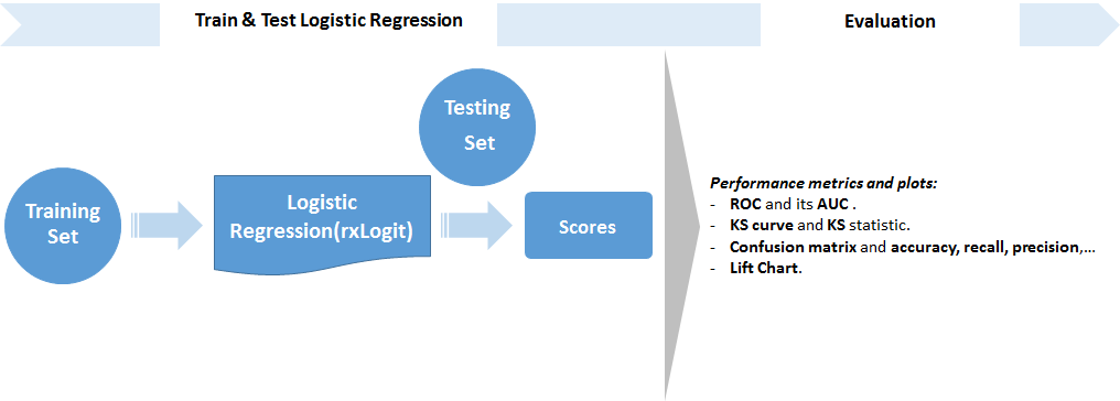
Step 3a: Training

In this step, we create a stored procedure [dbo].[train_model] that trains a Logistic Regression on the training set. The trained model is serialized and stored in a table called Model using an Odbc connection. Training a Logistic Regression for loan credit risk prediction is a standard practice in the Credit Score industry. Contrary to more complex models such as random forests or neural networks, it is easily understandable through the simple formula generated during the training. Also, the presence of bucketed numeric variables helps understand the impact of each category and variable on the probability of default. The variables used and their respective coefficients, sorted by order of magnitude, are stored in the table Logistic_Coeff.

Input:

• Merged_Features and Hash_Id tables.

Output:

• Model table containing the trained model.
• Logistic_Coeff table with variables names and coefficients of the logistic regression formula. They are sorted in decreasing order of the absolute value of the coefficients.

Related files:

• step3a_training.sql

Example

EXEC train_model 'Merged_Features'

Step 3b: Scoring

In this step, we create a stored procedure [dbo].[score] that scores the trained model on the testing set. The Predictions are stored in a SQL table.

Input:

• Merged_Features,Hash_Id, and Model tables.

Output:

• Predictions_Logistic table storing the predictions from the tested model.

Related files:

• step3b_scoring.sql

Example:

EXEC score 'SELECT * FROM Merged_Features WHERE loanId NOT IN (SELECT loanId from Hash_Id WHERE hashCode <= 70)', 'Predictions_Logistic'

Step 3c: Evaluating

In this step, we create a stored procedure [dbo].[evaluate] that computes classification performance metrics written in the table Metrics. The metrics are:

• KS (Kolmogorov-Smirnov) statistic. It is a standard performance metric in the credit score industry. It represents how well the model can differenciate between the Good Credit applicants from the Bad Credit applicants in the testing set.
• Various classification performance metrics computed on the confusion matrix. These are dependent on the threshold chosen to decide whether to classify a predicted probability as good or bad. Here, we use as a threshold the point on the x axis in the KS plot where the curves are the farthest possible.
• AUC (Area Under the Curve) for the ROC. It represents how well the model can differenciate between the Good Credit applicants from the Bad Credit applicants given a good decision threshold in the testing set.

Input:

• Predictions_Logistic table storing the predictions from the tested model.

Output:

• Metrics table containing the performance metrics of the model.

Related files:

• step3c_evaluating.sql

Example:

EXEC evaluate 'Predictions_Logistic'

Step 4: Operational Metrics Computation and Scores Transformation

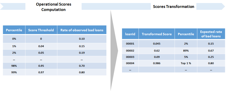
In this step, we create two stored procedures [dbo].[compute_operational_metrics], and [apply_score_transformation].

The first, [dbo].[compute_operational_metrics] will:

1. Apply a sigmoid function to the output scores of the logistic regression, in order to spread them in [0,1] and make them more interpretable. This sigmoid uses the average predicted score, so it is saved into the table Scores_Average for use in the Production pipeline.

2. Compute bins for the scores, based on quantiles (we compute the 1%-99% percentiles).

3. Take each lower bound of each bin as a decision threshold for default loan classification, and compute the rate of bad loans among loans with a score higher than the threshold.

It outputs the table Operational_Metrics, which will also be used in the Production pipeline. It can be read in the following way:

• If the score cutoff of the 91th score percentile is 0.9834, and we read a bad rate of 0.6449, this means that if 0.9834 is used as a threshold to classify loans as bad, we would have a bad rate of 64.49%. This bad rate is equal to the number of observed bad loans over the total number of loans with a score greater than the threshold.

The second, [apply_score_transformation] will:

1. Apply the same sigmoid function to the output scores of the logistic regression, in order to spread them in [0,1].

2. Asssign each score to a percentile bin with the bad rates given by the Operational_Metrics table. These bad rates are either observed (Modeling pipeline) or expected (Production pipeline).

Input:

• Predictions_Logistic table storing the predictions from the tested model.

Output:

• Operational_Metrics table containing the percentiles from 1% to 99%, the scores thresholds each one corresponds to, and the observed bad rate among loans with a score higher than the corresponding threshold.
• Scores_Average table containing the single value of the average score output from the logistic regression. It is used for the sigmoid transformation in Modeling and Production pipeline.
• Scores table containing the transformed scores for each record of the testing set, together with the percentiles they belong to, the corresponding score cutoff, and the observed bad rate among loans with a higher score than this cutoff.

Related files:

• step4_operational_metrics.sql

Example:

EXEC compute_operational_metrics 'Predictions_Logistic'
EXEC apply_score_transformation 'Predictions_Logistic', 'Scores'

The Production Pipeline

In the Production pipeline, the data from the files Loan_Prod.csv and Borrower_Prod.csv is uploaded through PowerShell to the Loan_Prod and Borrower_Prod tables.

The Loan_Prod and Borrower_Prod tables are then merged and cleaned like in Step 1 (using the Stats table), and a feature engineered table is created like in Step 2 (using the Bins table). The featurized table is then scored on the logistic regression model (using the Model and Column_Info tables). Finally, the scores are transformed and stored in the Scores_Prod table (using the Scores_Average and Operational_Metrics tables).

Example:

EXEC merging 'Loan_Prod', 'Borrower_Prod', 'Merged_Prod'
EXEC fill_NA_mode_mean 'Merged_Prod', 'Merged_Cleaned_Prod'
EXEC feature_engineering 'Merged_Cleaned_Prod', 'Merged_Features_Prod'
EXEC score 'SELECT * FROM Merged_Features_Prod', 'Predictions_Logistic_Prod'
exec apply_score_transformation 'Predictions_Logistic_Prod', 'Scores_Prod'
ALTER TABLE Scores_Prod DROP COLUMN isBad