Track Predictions for Typhoon Nanmadol#
In this example, we will download HRES T0 data for 17 Sep 2022 from WeatherBench2 at 0.25 degrees resolution and use this as an initial condition to predict the track Typhoon Nanmadol.
Running this notebook requires additional Python packages. You can install these as follows:
pip install gcsfs cdsapi zarr matplotlib
Downloading the Data#
To begin with, we download the data from WeatherBench2.
from pathlib import Path

import fsspec
import xarray as xr

# Data will be downloaded here.
download_path = Path("~/downloads/tc_tracking")

download_path = download_path.expanduser()
download_path.mkdir(parents=True, exist_ok=True)

# We will download from Google Cloud.
url = "gs://weatherbench2/datasets/hres_t0/2016-2022-6h-1440x721.zarr"
ds = xr.open_zarr(fsspec.get_mapper(url), chunks=None)

# Day to download. This will download all times for that day.
day = "2022-09-17"

# Download the surface-level variables. We write the downloaded data to another file to cache.
if not (download_path / f"{day}-surface-level.nc").exists():
    surface_vars = [
        "10m_u_component_of_wind",
        "10m_v_component_of_wind",
        "2m_temperature",
        "mean_sea_level_pressure",
    ]
    ds_surf = ds[surface_vars].sel(time=day).compute()
    ds_surf.to_netcdf(str(download_path / f"{day}-surface-level.nc"))
print("Surface-level variables downloaded!")

# Download the atmospheric variables. We write the downloaded data to another file to cache.
if not (download_path / f"{day}-atmospheric.nc").exists():
    atmos_vars = [
        "temperature",
        "u_component_of_wind",
        "v_component_of_wind",
        "specific_humidity",
        "geopotential",
    ]
    ds_atmos = ds[atmos_vars].sel(time=day).compute()
    ds_atmos.to_netcdf(str(download_path / f"{day}-atmospheric.nc"))
print("Atmos-level variables downloaded!")
Surface-level variables downloaded!
Atmos-level variables downloaded!
Downloading Static Variables from ERA5 Data#
The static variables are not available in WeatherBench2, so we need to download them from ERA5, just like we did in the example for ERA5.
To do so, register an account with the Climate Data Store and create $HOME/.cdsapirc with the following content:
url: https://cds.climate.copernicus.eu/api
key: <API key>
You can find your API key on your account page.
In order to be able to download ERA5 data, you need to accept the terms of use in the dataset page.
from pathlib import Path

import cdsapi

c = cdsapi.Client()

# Download the static variables.
if not (download_path / "static.nc").exists():
    c.retrieve(
        "reanalysis-era5-single-levels",
        {
            "product_type": "reanalysis",
            "variable": [
                "geopotential",
                "land_sea_mask",
                "soil_type",
            ],
            "year": "2023",
            "month": "01",
            "day": "01",
            "time": "00:00",
            "format": "netcdf",
        },
        str(download_path / "static.nc"),
    )
print("Static variables downloaded!")
2025-05-08 10:03:42,563 INFO [2024-09-26T00:00:00] Watch our [Forum](https://forum.ecmwf.int/) for Announcements, news and other discussed topics.
2025-05-08 10:03:42,564 WARNING [2024-06-16T00:00:00] CDS API syntax is changed and some keys or parameter names may have also changed. To avoid requests failing, please use the "Show API request code" tool on the dataset Download Form to check you are using the correct syntax for your API request.
Static variables downloaded!
Preparing a Batch#
We convert the downloaded data to an aurora.Batch, which is what the model requires.
import numpy as np
import torch
import xarray as xr

from aurora import Batch, Metadata

static_vars_ds = xr.open_dataset(download_path / "static.nc", engine="netcdf4")
surf_vars_ds = xr.open_dataset(download_path / f"{day}-surface-level.nc", engine="netcdf4")
atmos_vars_ds = xr.open_dataset(download_path / f"{day}-atmospheric.nc", engine="netcdf4")


def _prepare(x: np.ndarray) -> torch.Tensor:
    """Prepare a variable.

    This does the following things:
    * Select time points two and three: hours 06:00 and 12:00.
    * Insert an empty batch dimension with `[None]`.
    * Flip along the latitude axis to ensure that the latitudes are decreasing.
    * Copy the data, because the data must be contiguous when converting to PyTorch.
    * Convert to PyTorch.
    """
    return torch.from_numpy(x[[1, 2]][None][..., ::-1, :].copy())


batch = Batch(
    surf_vars={
        "2t": _prepare(surf_vars_ds["2m_temperature"].values),
        "10u": _prepare(surf_vars_ds["10m_u_component_of_wind"].values),
        "10v": _prepare(surf_vars_ds["10m_v_component_of_wind"].values),
        "msl": _prepare(surf_vars_ds["mean_sea_level_pressure"].values),
    },
    static_vars={
        # The static variables are constant, so we just get them for the first time. They
        # don't need to be flipped along the latitude dimension, because they are from
        # ERA5.
        "z": torch.from_numpy(static_vars_ds["z"].values[0]),
        "slt": torch.from_numpy(static_vars_ds["slt"].values[0]),
        "lsm": torch.from_numpy(static_vars_ds["lsm"].values[0]),
    },
    atmos_vars={
        "t": _prepare(atmos_vars_ds["temperature"].values),
        "u": _prepare(atmos_vars_ds["u_component_of_wind"].values),
        "v": _prepare(atmos_vars_ds["v_component_of_wind"].values),
        "q": _prepare(atmos_vars_ds["specific_humidity"].values),
        "z": _prepare(atmos_vars_ds["geopotential"].values),
    },
    metadata=Metadata(
        # Flip the latitudes! We need to copy because converting to PyTorch, because the
        # data must be contiguous.
        lat=torch.from_numpy(surf_vars_ds.latitude.values[::-1].copy()),
        lon=torch.from_numpy(surf_vars_ds.longitude.values),
        # Converting to `datetime64[s]` ensures that the output of `tolist()` gives
        # `datetime.datetime`s. Note that this needs to be a tuple of length one:
        # one value for every batch element. Select the third time point.
        time=(surf_vars_ds.time.values.astype("datetime64[s]").tolist()[2],),
        atmos_levels=tuple(int(level) for level in atmos_vars_ds.level.values),
    ),
)
Loading and Running the Model#
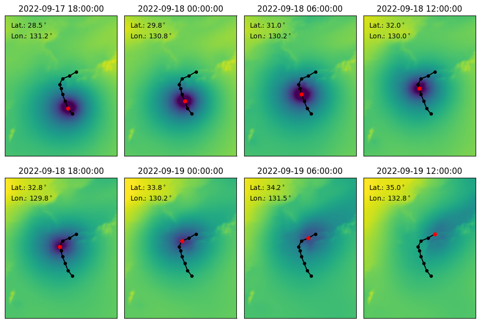
Finally, we are ready to load and run the model and visualise the predictions. We perform a roll-out for eight steps, which produces predictions for up to two days into the future.
The model can be run locally, or run on Azure AI Foundry. To run on Foundry, the environment variables FOUNDRY_ENDPOINT, FOUNDRY_TOKEN, and BLOB_URL_WITH_SAS need to be set. If you’re unsure on how to set environment variables, see here.
from datetime import datetime

from aurora import Tracker

# Initialise the tracker with the position of Nanmadol at 17 Sept 2022 at UTC 12. Taken from
# IBTrACS: https://ncics.org/ibtracs/index.php?name=v04r01-2022254N24143
tracker = Tracker(init_lat=27.50, init_lon=132, init_time=datetime(2022, 9, 17, 12, 0))

# Set to `False` to run locally and to `True` to run on Foundry.
run_on_foundry = False
if not run_on_foundry:
    from aurora import Aurora, Tracker, rollout

    model = Aurora()
    model.load_checkpoint("microsoft/aurora", "aurora-0.25-finetuned.ckpt")

    model.eval()
    model = model.to("cuda")

    preds = []
    with torch.inference_mode():
        for pred in rollout(model, batch, steps=8):
            pred = pred.to("cpu")  # Immediately free up the GPU.
            preds.append(pred)
            tracker.step(pred)

    model = model.to("cpu")
if run_on_foundry:
    import logging
    import os
    import warnings

    from aurora.foundry import BlobStorageChannel, FoundryClient, submit

    # In this demo, we silence all warnings.
    warnings.filterwarnings("ignore")

    # But we do want to show what's happening under the hood!
    logging.basicConfig(level=logging.WARNING, format="%(asctime)s [%(levelname)s] %(message)s")
    logging.getLogger("aurora").setLevel(logging.INFO)

    foundry_client = FoundryClient(
        endpoint=os.environ["FOUNDRY_ENDPOINT"],
        token=os.environ["FOUNDRY_TOKEN"],
    )
    channel = BlobStorageChannel(os.environ["BLOB_URL_WITH_SAS"])

    for pred in submit(
        batch,
        model_name="aurora-0.25-finetuned",
        num_steps=8,
        foundry_client=foundry_client,
        channel=channel,
    ):
        preds.append(pred)
        tracker.step(pred)
import matplotlib.pyplot as plt

track = tracker.results()

fig, axs = plt.subplots(2, 4, figsize=(10, 7))

for i in range(8):
    pred = preds[i]
    ax = axs[i // 4, i % 4]

    # Cut a square around Nanmadol.
    lat_mask = (pred.metadata.lat >= 20) & (pred.metadata.lat <= 45)
    lon_mask = (pred.metadata.lon >= 120) & (pred.metadata.lon <= 140)

    # Show the forecast for MSL.
    ax.imshow(
        pred.surf_vars["msl"][0, 0][lat_mask][:, lon_mask].numpy() / 100,
        vmin=970,
        vmax=1020,
        extent=(120, 140, 20, 45),
    )
    ax.set_title(str(pred.metadata.time[0]))
    ax.set_xticks([])
    ax.set_yticks([])

    # Plot the whole track for Typhoon Nanmadol.
    ax.plot(track.lon, track.lat, c="k", marker=".", markersize=8)

    # Highlight the current step and also display it on the top left.
    this_step = track[track.time == pred.metadata.time[0]]
    ax.plot(this_step.lon, this_step.lat, c="r", marker=".", markersize=10)
    ax.text(
        0.05,
        0.95,
        f"Lat.: {this_step.lat.iloc[0]:.1f}${{}}^\\circ$",
        ha="left",
        va="top",
        transform=ax.transAxes,
    )
    ax.text(
        0.05,
        0.875,
        f"Lon.: {this_step.lon.iloc[0]:.1f}${{}}^\\circ$",
        ha="left",
        va="top",
        transform=ax.transAxes,
    )

plt.tight_layout()