Typical Workflow
This solution template demonstrates a solution end to end to run predictive analytics on loan data and produce scoring on chargeoff probability. A PowerBI report will also walk through the analysis and trend of credit loans and prediction of chargeoff probability.
To demonstrate a typical workflow, we’ll introduce you to a few personas. You can follow along by performing the same steps for each persona.
If you want to follow along and have *not* run the PowerShell script, you must to first create a database table in your SQL Server. You will then need to replace the connection_string at the top of each R file with your database and login information.
Step 1: Server Setup and Configuration with Danny the DB Analyst Ivan the IT Administrator
This step has already been done on your 'Deploy to Azure' VM.
You can perform these steps in your environment by using the instructions to Setup your On-Prem SQL Server.
The cluster has been created and data loaded for you when you used the Deploy button on the Quick Start page. Once you complete the walkthrough, you will want to delete this cluster as it incurs expense whether it is in use or not - see HDInsight Cluster Maintenance for more details.
Step 2: Data Prep and Modeling with Debra the Data Scientist
Now let’s meet Debra, the Data Scientist. Debra’s job is to use loan payment data to predict loan chargeoff risk. Debra’s preferred language for developing the models is using R and SQL. She uses Microsoft ML Services with SQL Server 2017 as it provides the capability to run large datasets and also is not constrained by memory restrictions of Open Source R.Debra will develop these models using HDInsight, the managed cloud Hadoop solution with integration to Microsoft ML Server.
After analyzing the data she opted to create multiple models and choose the best one. She will create five machine learning models and compare them, then use the one she likes best to compute a prediction for each loan, and then select the loan with the highest probability of chargeoff.
http://CLUSTERNAME.azurehdinsight.net/rstudio.
library(RevoScaleR)
library(MicrosoftML)
library(xgboost)

# spark cc object
sparkContext <- rxSparkConnect(consoleOutput = TRUE, reset = TRUE)

# set compute context to local
rxSetComputeContext('local')

# Copy model rds files to local dev folder from HDFS
LocalDir <- paste("/var/RevoShare/", Sys.info()[["user"]], "/LoanChargeOff/dev/model/", sep="" )
if(!dir.exists(LocalDir)){
   system(paste("mkdir -p -m 777 ", LocalDir, sep="")) # create a new directory
}
RemoteFiles <- "/LoanChargeOff/model/*.rds"
rxHadoopCopyToLocal(source = RemoteFiles, dest = LocalDir)

# clean up
rm(list = ls())
</div>
Solution Explorer tab on the right. In RStudio, the files can be found in the Files tab, also on the right.
- Step 1: Creating Tables
- Step 2: Creating Views with Features and Labels
- Step 2a: Demonstrate feature selection using MicrosoftML package
- Step 3: Training and Testing Model
- Step 4: Chargeoff Prediction (batch)
- Step 4a: Chargeoff Prediction (OnDemand)
-
loanchargeoff_main.R is used to define the data and directories and then run all of the steps to process data, perform feature engineering, training, and scoring.
The default input for this script uses 100,000 loans for training models, and will split this into train and test data. After running this script you will see data files in the /LoanChargeOff/dev/temp directory on your storage account. Models are stored in the /LoanChargeOff/dev/model directory on your storage account. The Hive table
loanchargeoff_predictionscontains the 100,000 records with predictions (Score,Probability) created from the best model. - Copy_Dev2Prod.R copies the model information from the dev folder to the prod folder to be used for production. This script must be executed once after loanchargeoff_main.R completes, before running loanchargeoff_scoring.R. It can then be used again as desired to update the production model. After running this script models created during loanchargeoff_main.R are copied into the /var/RevoShare/user/LoanChargeOff/prod/model directory.
-
loanchargeoff_scoring.R uses the previously trained model and invokes the steps to process data, perform feature engineering and scoring. Use this script after first executing loanchargeoff_main.R and Copy_Dev2Prod.R.
The input to this script defaults to 10,000 loans to be scored with the model in the prod directory. After running this script the Hive table
loanchargeoff_predictionsnow contains the predictions.
- step1_get_training_testing_data.R: Read input data which contains all the history information for all the loans from HDFS. Extract training/testing data based on process date (paydate) from the input data. Save training/testing data in HDFS working directory
- step2_feature_engineering.R: Here we use MicrosoftML to do feature selection. Code can be added in this file to create some new features based on existing features. Open source package such as Caret can also be used to do feature selection here. Best features are selected using AUC.
- Now she is ready for training the models, using step3_training_evaluation.R. This step will train two different models and evaluate each.
The R script draws the ROC or Receiver Operating Characteristic for each prediction model. It shows the performance of the model in terms of true positive rate and false positive rate, when the decision threshold varies.
The AUC is a number between 0 and 1. It corresponds to the area under the ROC curve. It is a performance metric related to how good the model is at separating the two classes (converted clients vs. not converted), with a good choice of decision threshold separating between the predicted probabilities. The closer the AUC is to 1, and the better the model is. Given that we are not looking for that optimal decision threshold, the AUC is more representative of the prediction performance than the Accuracy (which depends on the threshold).
Debra will use the AUC to select the champion model to use in the next step.
- step4_prepare_new_data.R creates a new data which contains all the opened loans on a pay date which we do not know the status in next three month, the loans in this new data are not included in the training and testing dataset and have the same features as the loans used in training/testing dataset.
- step5_loan_prediction.R takes the new data created in the step4 and the champion model created in step3, output the predicted label and probability to be charge-off for each loan in next three months.
- loanchargeoff_xgboost.R This step is optional. For more details : Using XGBoost package in HDInsight Spark Cluster for Loan ChargeOff Prediction
- After creating the model, Debra runs Copy_Dev2Prod.R to copy the model information from the dev folder to the prod folder, then runs loanchargeoff_scoring.R to create predictions for her new data.
- Once all the above code has been executed, Debra will use PowerBI to visualize the recommendations created from her model.
She uses an ODBC connection to connect to the data, so that it will always show the most recently modeled and scored data.
You can access this dashboard in either of the following ways:
-
Open the PowerBI file from the D:\LoanChargeOffSolution\Reports directory on the deployed VM desktop.
-
Install PowerBI Desktop on your computer and download and open the Loan ChargeOff Prediction Dashboard
-
Install PowerBI Desktop on your computer and download and open the Loan ChargeOff Prediction HDI Dashboard
 If you want to refresh data in your PowerBI Dashboard, make sure to follow these instructions to setup and use an ODBC connection to the dashboard.
 -
- A summary of this process and all the files involved is described in more detail here.
Step 3: Operationalize with Debra and Danny
Debra has completed her tasks. She has connected to the SQL database, executed code from her R IDE that pushed (in part) execution to the SQL machine to clean the data, create new features, train five models and select the champion model.She has executed code from RStudio that pushed (in part) execution to Hadoop to clean the data, create new features, train five models and select the champion model She has scored data, created predictions, and also created a summary report which she will hand off to Bernie - see below. While this task is complete for the current set of loans, our company will want to perform these actions for each new loan payment. Instead of going back to Debra each time, Danny can operationalize the code in TSQL files which he can then run himself each month for the newest loan payments.
Programmability>Stored Procedures section of the LoanChargeOff database.
 Log into SSMS using SQL Server Authentication - the username/password provided during deployment
You can find this script in the SQLR directory, and execute it yourself by following the PowerShell Instructions.
As noted earlier, this was already executed when your VM was first created. As noted earlier, this is the fastest way to execute all the code included in this solution. (This will re-create the same set of tables and models as the above R scripts.)
Log into SSMS using SQL Server Authentication - the username/password provided during deployment
You can find this script in the SQLR directory, and execute it yourself by following the PowerShell Instructions.
As noted earlier, this was already executed when your VM was first created. As noted earlier, this is the fastest way to execute all the code included in this solution. (This will re-create the same set of tables and models as the above R scripts.)
Step 4: Deploy and Visualize with Bernie the Business Analyst
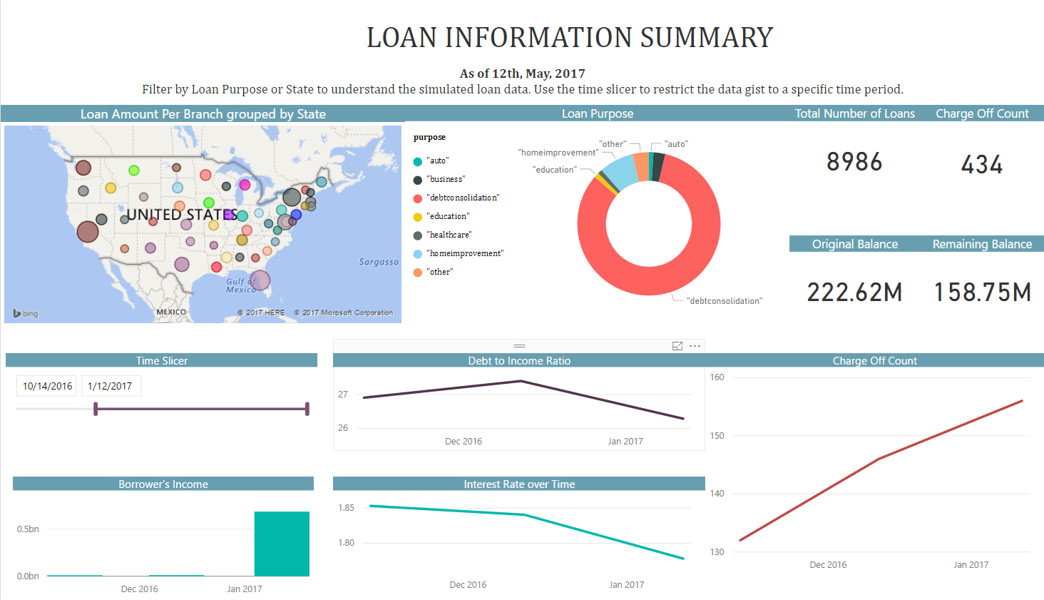
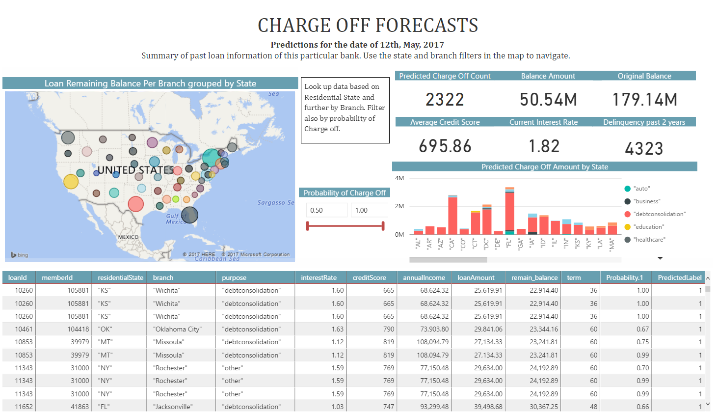
Now that the predictions are created and saved, we will meet our last persona - Bernie, the Business Analyst. Bernie will use the Power BI Dashboard to learn more about the loan chargeoff predictions (second tab). He will also review summaries of the loan data used to create the model (first tab).
You can access this dashboard in either of the following ways:
-
Open the PowerBI file from the D:\LoanChargeOffSolution\Reports directory on the deployed VM desktop.
-
Install PowerBI Desktop on your computer and download and open the Loan ChargeOff Prediction Dashboard
-
Install PowerBI Desktop on your computer and download and open the Loan ChargeOff Prediction HDI Dashboard