import pandas as pd
import numpy as np
import uci_dataset as database
import torch

import raimitigations.dataprocessing as dp
from raimitigations.utils import split_data, train_model_plot_results

Case Study 1

This notebook shows an example of how to use the dataprocessing library. Here, we show how to use this library to explore and transform a dataset with the goal to improve a model’s accuracy. Here, we will work with the breast cancer dataset. The dataset is automatically fetched by using the uci_dataset library.

Fixing a seed

To avoid randomness in the following experiments, we’ll fix the seeds to guarantee that the results obtained are the same each time we run this notebook. Feel free to comment the next cell or test different seeds to see how this affects the results.

import random
SEED = 45
np.random.seed(SEED)
random.seed(SEED)
torch.manual_seed(SEED)

<torch._C.Generator at 0x7f25279f79f0>

1 - Understanding the Data

df = database.load_breast_cancer()
label_col = "Class"
df

	Class	age	menopause	tumor-size	inv-nodes	node-caps	deg-malig	breast	breast-quad	irradiat
0	no-recurrence-events	30-39	premeno	30-34	0-2	no	3	left	left_low	no
1	no-recurrence-events	40-49	premeno	20-24	0-2	no	2	right	right_up	no
2	no-recurrence-events	40-49	premeno	20-24	0-2	no	2	left	left_low	no
3	no-recurrence-events	60-69	ge40	15-19	0-2	no	2	right	left_up	no
4	no-recurrence-events	40-49	premeno	0-4	0-2	no	2	right	right_low	no
...	...	...	...	...	...	...	...	...	...	...
281	recurrence-events	30-39	premeno	30-34	0-2	no	2	left	left_up	no
282	recurrence-events	30-39	premeno	20-24	0-2	no	3	left	left_up	yes
283	recurrence-events	60-69	ge40	20-24	0-2	no	1	right	left_up	no
284	recurrence-events	40-49	ge40	30-34	3-5	no	3	left	left_low	no
285	recurrence-events	50-59	ge40	30-34	3-5	no	3	left	left_low	no

286 rows × 10 columns

df.info()

<class 'pandas.core.frame.DataFrame'>
RangeIndex: 286 entries, 0 to 285
Data columns (total 10 columns):
 #   Column       Non-Null Count  Dtype
---  ------       --------------  -----
 0   Class        286 non-null    object
 1   age          286 non-null    object
 2   menopause    286 non-null    object
 3   tumor-size   286 non-null    object
 4   inv-nodes    286 non-null    object
 5   node-caps    278 non-null    object
 6   deg-malig    286 non-null    int64
 7   breast       286 non-null    object
 8   breast-quad  285 non-null    object
 9   irradiat     286 non-null    object
dtypes: int64(1), object(9)
memory usage: 22.5+ KB

There are several categorical data in this dataset. Actually, only one feature is numeric, while the remaining columns are all categorical. Therefore, we should take a closer look at each column in order to determine which encoding method should be used to each one. From the summary of the dataset, presented two cells up, we notice that many of the categorical classes doesn’t present any order. For these, we should use One-Hot encoding. However, some of these columns present some order among their categories. For example, the age column presents a hierarchical information. Let’s take a look a these ordered categorical data:

print(f"age unique values = {df['age'].unique()}")
print(f"tumor-size unique values = {df['tumor-size'].unique()}")
print(f"inv-nodes unique values = {df['inv-nodes'].unique()}")

age unique values = ['30-39' '40-49' '60-69' '50-59' '70-79' '20-29']
tumor-size unique values = ['30-34' '20-24' '15-19' '0-4' '25-29' '50-54' '10-14' '40-44' '35-39'
 '5-9' '45-49']
inv-nodes unique values = ['0-2' '6-8' '9-11' '3-5' '15-17' '12-14' '24-26']

After a few cells, we will use this information when encoding our data.

Before modifying the dataset, let’s analyze the correlations within its columns. To do that, let’s use the CorrelatedFeatures class, which computes the correlation between numerical x numerical, categorical x numerical, and categorical x categorical data. Please refer to the notebook in notebooks/module_tests/feat_sel_corr_tutorial.ipynb for an in depth analysis of this class. In a nutshell: this class will compute the correlation between all pairs of variables (or we can look only to a specific set of variables if needed) and remove one variable for each pair of correlated variables. This class uses a fit method to compute the correlations and a transform method to effectively remove the correlated variables. For now, we are only interested in analysing the correlations between the columns. We will save the results found by this class in the files specified by json_summary, json_corr, and json_uncorr, respectively.

cor_feat = dp.CorrelatedFeatures(
                                    method_num_num=["spearman", "pearson", "kendall"],                              # Used for Numerical x Numerical correlations
                                    num_corr_th=0.9,                                                                                                # Used for Numerical x Numerical correlations
                                    num_pvalue_th=0.05,                                                                                             # Used for Numerical x Numerical correlations
                                    method_num_cat="model",                                                                                 # Used for Numerical x Categorical correlations
                                    model_metrics=["f1", "auc"],                                                                    # Used for Numerical x Categorical correlations
                                    metric_th=0.9,                                                                                                  # Used for Numerical x Categorical correlations
                                    cat_corr_th=0.9,                                                                                                # Used for Categorical x Categorical correlations
                                    cat_pvalue_th=0.01,                                                                                             # Used for Categorical x Categorical correlations
                                    json_summary="./corr_json/c1_summary.json",
                                    json_corr="./corr_json/c1_corr.json",
                                    json_uncorr="./corr_json/c1_uncorr.json"
                            )
cor_feat.fit(df=df, label_col=label_col)

No correlations detected. Nothing to be done here.

<raimitigations.dataprocessing.feat_selection.correlated_features.CorrelatedFeatures at 0x7f259488ba00>

Remember to look through the JSON files generated in the previous cell.

2 - Basic Pre-Processing

Encode Categorical Variables

The next step is crucial for preparing our dataset so it can be used by a model. As previously mentioned, we will encode the data using two encoding methods: ordinal encoding for categorical columns with ordered categories, and one-hot encoding for unordered categorical data. The columns “age”, “tumor-size”, “inv-nodes”, and “Class” will all be encoded using ordinal encoding. For the “age”, “tumor-size”, and “inv-nodes” columns, we provide a list with the ordered categories, which shows the encoder how it should order the encoding numbers (lower values will be associated to the initial categories, while higher encoding values will be associated to the final categories). After creating the encoder object from the EncoderOrdinal class, we call its fit method while passing the dataset df to it. We then call the transform method, which returns a new copy of the dataset with the categorical columns specified encoded using ordinal encoding. We then proceed to perform the one-hot encoding by instantiating an object of class EncoderOHE and then calling its fit and transform methods.

# Set the order that the ordinal encoder should use
age_order = df['age'].unique()
age_order.sort()
tumor_size_order = df['tumor-size'].unique()
tumor_size_order.sort()
inv_nodes_order = df['inv-nodes'].unique()
inv_nodes_order.sort()

# Encode 'tumor-size', 'Class', and 'inv-nodes' using ordinal encoding
enc_ord = dp.EncoderOrdinal(col_encode=["age", "tumor-size", "inv-nodes", "Class"],
                                                    categories={"age":age_order,
                                                                            "tumor-size":tumor_size_order,
                                                                            "inv-nodes":inv_nodes_order}
                                            )
enc_ord.fit(df)
proc_df = enc_ord.transform(df)

# Encode the remaining categorical columns using One-Hot Encoding
enc_ohe = dp.EncoderOHE()
enc_ohe.fit(proc_df)
proc_df = enc_ohe.transform(proc_df)
proc_df

No columns specified for encoding. These columns have been automatically identfied as the following:
['menopause', 'node-caps', 'breast', 'breast-quad', 'irradiat']

	Class	age	tumor-size	inv-nodes	deg-malig	menopause_lt40	menopause_premeno	node-caps_yes	node-caps_nan	breast_right	breast-quad_left_low	breast-quad_left_up	breast-quad_right_low	breast-quad_right_up	breast-quad_nan	irradiat_yes
0	0	1	5	0	3	0	1	0	0	0	1	0	0	0	0	0
1	0	2	3	0	2	0	1	0	0	1	0	0	0	1	0	0
2	0	2	3	0	2	0	1	0	0	0	1	0	0	0	0	0
3	0	4	2	0	2	0	0	0	0	1	0	1	0	0	0	0
4	0	2	0	0	2	0	1	0	0	1	0	0	1	0	0	0
...	...	...	...	...	...	...	...	...	...	...	...	...	...	...	...	...
281	1	1	5	0	2	0	1	0	0	0	0	1	0	0	0	0
282	1	1	3	0	3	0	1	0	0	0	0	1	0	0	0	1
283	1	4	3	0	1	0	0	0	0	1	0	1	0	0	0	0
284	1	2	5	4	3	0	0	0	0	0	1	0	0	0	0	0
285	1	3	5	4	3	0	0	0	0	0	1	0	0	0	0	0

286 rows × 16 columns

We can now check that our dataset has only numerical columns in it.

proc_df.info()

<class 'pandas.core.frame.DataFrame'>
RangeIndex: 286 entries, 0 to 285
Data columns (total 16 columns):
 #   Column                 Non-Null Count  Dtype
---  ------                 --------------  -----
 0   Class                  286 non-null    int64
 1   age                    286 non-null    int64
 2   tumor-size             286 non-null    int64
 3   inv-nodes              286 non-null    int64
 4   deg-malig              286 non-null    int64
 5   menopause_lt40         286 non-null    int32
 6   menopause_premeno      286 non-null    int32
 7   node-caps_yes          286 non-null    int32
 8   node-caps_nan          286 non-null    int32
 9   breast_right           286 non-null    int32
 10  breast-quad_left_low   286 non-null    int32
 11  breast-quad_left_up    286 non-null    int32
 12  breast-quad_right_low  286 non-null    int32
 13  breast-quad_right_up   286 non-null    int32
 14  breast-quad_nan        286 non-null    int32
 15  irradiat_yes           286 non-null    int32
dtypes: int32(11), int64(5)
memory usage: 23.6 KB

Impute Missing Data and Split Dataset

The next step consists on doing the following:

• split the dataset into train and test sets;

• impute any missing data (if any).

train_x, test_x, train_y, test_y = split_data(proc_df, label_col, test_size=0.25)

imputer = dp.BasicImputer()
imputer.fit(train_x)
train_x = imputer.transform(train_x)
test_x = imputer.transform(test_x)
train_x

No columns specified for imputation. These columns have been automatically identified:
[]

	age	tumor-size	inv-nodes	deg-malig	menopause_lt40	menopause_premeno	node-caps_yes	node-caps_nan	breast_right	breast-quad_left_low	breast-quad_left_up	breast-quad_right_low	breast-quad_right_up	breast-quad_nan	irradiat_yes
165	2	3	4	2	0	1	0	0	1	0	1	0	0	0	0
79	2	4	0	2	0	1	0	0	1	0	0	0	0	0	0
278	3	6	2	3	0	1	1	0	1	0	0	0	1	0	0
247	3	5	6	3	0	0	1	0	0	0	0	1	0	0	1
248	4	6	5	3	0	0	1	0	0	1	0	0	0	0	0
...	...	...	...	...	...	...	...	...	...	...	...	...	...	...	...
217	2	2	0	2	0	1	0	0	0	0	1	0	0	0	0
135	1	3	4	2	0	1	0	0	1	0	0	0	0	0	0
258	3	5	5	2	0	0	1	0	0	0	0	1	0	0	1
78	3	4	0	2	0	1	0	0	0	1	0	0	0	0	0
164	4	4	4	1	0	0	0	1	1	1	0	0	0	0	1

214 rows × 15 columns

As we can see, the dataset didn’t have any missing values. Therefore, the BasicImputer didn’t do anything.

3 - Baseline Models

In the following cells, we train different models and plot their results over the test set. These models will be considered our baseline models. We will test 2 models as our baseline: XGBoost and K-Nearest Neighbors (KNN).

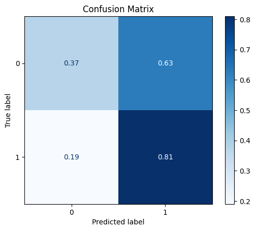
model = train_model_plot_results(train_x, train_y, test_x, test_y, model="xgb", train_result=False, plot_pr=False)

TEST SET:

[[26 25]
 [ 4 17]]

ROC AUC: 0.704014939309057
Precision: 0.6357142857142857
Recall: 0.6596638655462185
F1: 0.5908289241622575
Accuracy: 0.5972222222222222
Optimal Threshold (ROC curve): 0.2437402755022049
Optimal Threshold (Precision x Recall curve): 0.2437402755022049
Threshold used: 0.2437402755022049

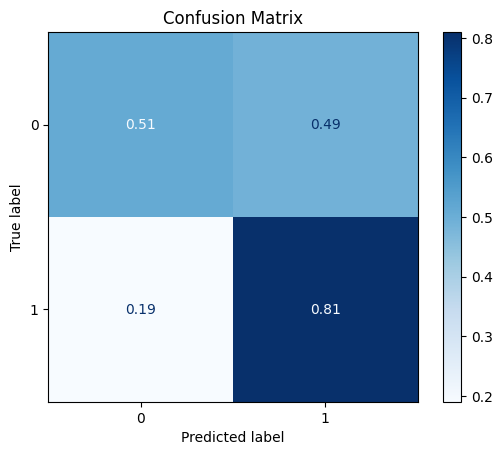
model = train_model_plot_results(train_x, train_y, test_x, test_y, model="knn", train_result=False, plot_pr=False)

TEST SET:

[[19 32]
 [ 4 17]]

ROC AUC: 0.6087768440709618
Precision: 0.5865128660159716
Recall: 0.5910364145658263
F1: 0.49961389961389957
Accuracy: 0.5
Optimal Threshold (ROC curve): 0.2
Optimal Threshold (Precision x Recall curve): 0.2
Threshold used: 0.2

4 - Feature Selection

From this point on, we will try to improve (even if slightly) the results of the baseline models. But before jumping into these improvements, an important note: there is some randomness involved in the training process we showed so far due to two factors:

• the train and test split;

• the model’s training process might involve some randomness.

Therefore, if you re-run this notebook with different SEED values, you most probably will get different results. Given the small size of the dataset being used here, the split between train and test sets can be crucial for getting good results. This means that some seed values might have results considerably better than others. Keep that in mind when looking through these results and testing different seeds (try commenting the cell where we fix the random seeds to check how the results vary). To really test the efficiency of the preprocessing steps shown here, we could run the split and train steps several times and record the mean (and standard deviation) of the results (auc, f1, etc.). This would give us a more powerful result. We encourage the interested user to check the notebook called notebooks/case_study/case1_stat.ipynb, which is a notebook where we perform the test previously described.

Now, let’s get back to our more simple experiments. Since we are using the same train and test split used by the baseline models, then we are good to go. Our first preprocessing (not considering the encoding part and the imputations, since those are mandatory to run the baseline models) is feature selection. Here, we will try the feature selection using the CatBoost model by using the CatBoostSelection class. Remember that we must pass the training set to the fit method, and then call the transform method over the training and test sets. This way we don’t use any information of the test set for this step, avoiding data contamination.

feat_sel = dp.CatBoostSelection(steps=5, verbose=False)
feat_sel.fit(X=train_x, y=train_y)
train_x_sel = feat_sel.transform(train_x)
test_x_sel = feat_sel.transform(test_x)

/home/matheus/miniconda3/envs/rai/lib/python3.9/site-packages/catboost/core.py:1222: FutureWarning: iteritems is deprecated and will be removed in a future version. Use .items instead.
  self._init_pool(data, label, cat_features, text_features, embedding_features, pairs, weight,

Let’s print the selected features:

feat_sel.get_selected_features()

['tumor-size',
 'inv-nodes',
 'deg-malig',
 'menopause_lt40',
 'node-caps_nan',
 'breast-quad_right_up',
 'breast-quad_nan']

Now, let’s re-train the KNN model and see how the feature selection preprocessing step affects the results:

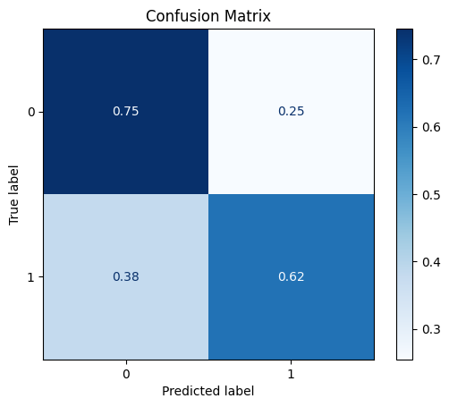
model = train_model_plot_results(train_x_sel, train_y, test_x_sel, test_y, model="knn", train_result=False, plot_pr=False)

TEST SET:

[[45  6]
 [14  7]]

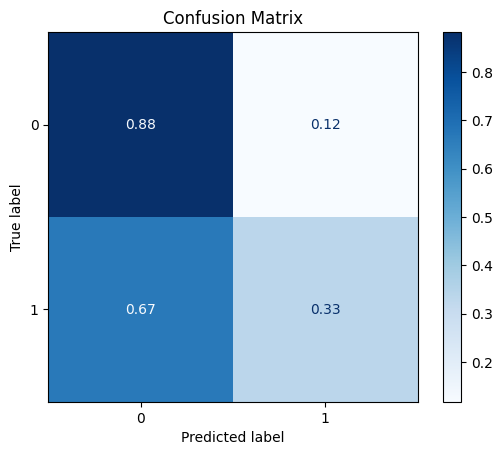
ROC AUC: 0.6321195144724556
Precision: 0.6505867014341591
Recall: 0.6078431372549019
F1: 0.6149732620320855
Accuracy: 0.7222222222222222
Optimal Threshold (ROC curve): 0.6
Optimal Threshold (Precision x Recall curve): 0.2
Threshold used: 0.6

Looking at the confusion matrix and comparing it to the baseline KNN model, we can see that the True Positives and True Negatives are now flipped. However, we did get an improvement on the other metrics. Therefore, using feature selection managed to improve the results while using less data (we are now using only 7 columns instead of 9).

5 - Synthetic Data

The next preprocessing step we will test is creating synthetic data. We will start by using SMOTE and its variations.

imblearn Library

The imblearn library implements several variations of SMOTE, a over sampling strategy, as well as some under sampling mehtods, such as TOMEK Links. The class Rebalance, present in the dataprocessing library, encapsulates the imblearn library and automates certain processes. For example, we don’t need to specify which version of SMOTE we want to use. We simply provide the dataset and specify the amount of new data we want, and the class Rebalance will do the rest: it will check the dataset and decide the best SMOTE variation to use, apply any under sampling method if requested, and run any preprocessing step if necessary (such as imputation). The user can also explicitly choose which SMOTE version they want by instantiating a SMOTE object (from imblearn) and passing it as a parameter to the Rebalance class. The same applies to the under sampling method.

Here, we use the default options provided by the Rebalance class regarding the SMOTE method. We choose to not use any under sampling method and we also specify explicitly the number of instances we want for the different values in the Y column.

train_y.value_counts()

0    150
1     64
Name: Class, dtype: int64

Since we got an improved performance when using feature selection, we’ll use our new dataset containing only the selected features in the following experiments. Note that these datasets are train_x and test_x.

rebalance = dp.Rebalance(
                            X=train_x_sel,
                            y=train_y,
                            strategy_over={0:150, 1:90},
                            over_sampler=True,
                            under_sampler=False
                    )
train_x_res, train_y_res = rebalance.fit_resample()
train_y_res.value_counts()

No columns specified for imputation. These columns have been automatically identified:
[]
Running oversampling...
...finished

0    150
1     90
Name: Class, dtype: int64

We can now retrain the KNN model using the new dataset with oversampling:

model = train_model_plot_results(train_x_res, train_y_res, test_x_sel, test_y, model="knn", train_result=False, plot_pr=False)

TEST SET:

[[44  7]
 [12  9]]

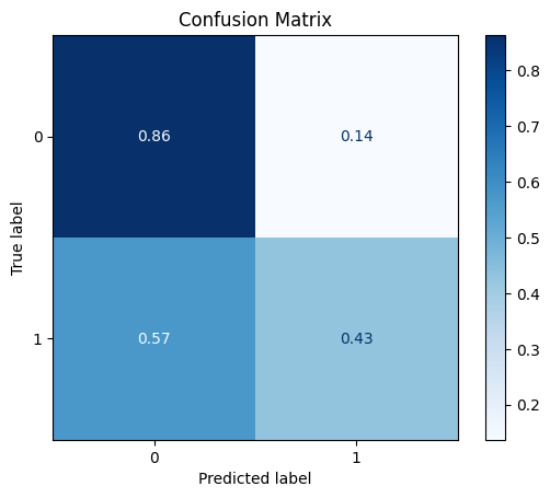
ROC AUC: 0.645658263305322
Precision: 0.6741071428571428
Recall: 0.6456582633053222
F1: 0.6544581965142713
Accuracy: 0.7361111111111112
Optimal Threshold (ROC curve): 0.6
Optimal Threshold (Precision x Recall curve): 0.6
Threshold used: 0.6

As we can see here, the oversampling managed to improve the results for the test set even further (compared to the feature selection step).

Creating Artificial Data using Deep Learning

Instead of using SMOTE to do the over sampling, we can also use Generator models to create artificial data similar to the ones observed in the training dataset.

CTGAN

In the next cell, we use the Synthesizer class to create artificial data using the CTGAN model. Similarly to what we’ve done in the Rebalance experiment, we’ll use the datasets produced by the feature selection step. We can also try training the CTGAN for more epochs and see how this affects the results.

synth = dp.Synthesizer(
                            X=train_x_sel,
                            y=train_y,
                            epochs=400,
                            model="ctgan",
                            load_existing=False
                    )

conditions = {label_col:1}
syn_train_x, syn_train_y = synth.fit_resample(X=train_x_sel, y=train_y, n_samples=20, conditions=conditions)
syn_train_y.value_counts()

/home/matheus/miniconda3/envs/rai/lib/python3.9/site-packages/sklearn/mixture/_base.py:131: ConvergenceWarning: Number of distinct clusters (7) found smaller than n_clusters (10). Possibly due to duplicate points in X.
  cluster.KMeans(
/home/matheus/miniconda3/envs/rai/lib/python3.9/site-packages/sklearn/mixture/_base.py:131: ConvergenceWarning: Number of distinct clusters (3) found smaller than n_clusters (10). Possibly due to duplicate points in X.
  cluster.KMeans(
/home/matheus/miniconda3/envs/rai/lib/python3.9/site-packages/ctgan/data_transformer.py:111: SettingWithCopyWarning:
A value is trying to be set on a copy of a slice from a DataFrame.
Try using .loc[row_indexer,col_indexer] = value instead

See the caveats in the documentation: https://pandas.pydata.org/pandas-docs/stable/user_guide/indexing.html#returning-a-view-versus-a-copy
  data[column_name] = data[column_name].to_numpy().flatten()
/home/matheus/miniconda3/envs/rai/lib/python3.9/site-packages/ctgan/data_transformer.py:111: SettingWithCopyWarning:
A value is trying to be set on a copy of a slice from a DataFrame.
Try using .loc[row_indexer,col_indexer] = value instead

See the caveats in the documentation: https://pandas.pydata.org/pandas-docs/stable/user_guide/indexing.html#returning-a-view-versus-a-copy
  data[column_name] = data[column_name].to_numpy().flatten()
/home/matheus/miniconda3/envs/rai/lib/python3.9/site-packages/ctgan/data_transformer.py:111: SettingWithCopyWarning:
A value is trying to be set on a copy of a slice from a DataFrame.
Try using .loc[row_indexer,col_indexer] = value instead

See the caveats in the documentation: https://pandas.pydata.org/pandas-docs/stable/user_guide/indexing.html#returning-a-view-versus-a-copy
  data[column_name] = data[column_name].to_numpy().flatten()
Sampling conditions:   0%|          | 0/20 [00:00<?, ?it/s]/home/matheus/miniconda3/envs/rai/lib/python3.9/site-packages/sdv/tabular/base.py:608: FutureWarning: In a future version of pandas, a length 1 tuple will be returned when iterating over a groupby with a grouper equal to a list of length 1. Don't supply a list with a single grouper to avoid this warning.
  for group, dataframe in grouped_conditions:
/home/matheus/miniconda3/envs/rai/lib/python3.9/site-packages/sdv/tabular/base.py:639: FutureWarning: In a future version of pandas, a length 1 tuple will be returned when iterating over a groupby with a grouper equal to a list of length 1. Don't supply a list with a single grouper to avoid this warning.
  for transformed_group, transformed_dataframe in transformed_groups:
/home/matheus/miniconda3/envs/rai/lib/python3.9/site-packages/ctgan/data_transformer.py:149: FutureWarning: In a future version, `df.iloc[:, i] = newvals` will attempt to set the values inplace instead of always setting a new array. To retain the old behavior, use either `df[df.columns[i]] = newvals` or, if columns are non-unique, `df.isetitem(i, newvals)`
  data.iloc[:, 1] = np.argmax(column_data[:, 1:], axis=1)
/home/matheus/miniconda3/envs/rai/lib/python3.9/site-packages/ctgan/data_transformer.py:149: FutureWarning: In a future version, `df.iloc[:, i] = newvals` will attempt to set the values inplace instead of always setting a new array. To retain the old behavior, use either `df[df.columns[i]] = newvals` or, if columns are non-unique, `df.isetitem(i, newvals)`
  data.iloc[:, 1] = np.argmax(column_data[:, 1:], axis=1)
/home/matheus/miniconda3/envs/rai/lib/python3.9/site-packages/ctgan/data_transformer.py:149: FutureWarning: In a future version, `df.iloc[:, i] = newvals` will attempt to set the values inplace instead of always setting a new array. To retain the old behavior, use either `df[df.columns[i]] = newvals` or, if columns are non-unique, `df.isetitem(i, newvals)`
  data.iloc[:, 1] = np.argmax(column_data[:, 1:], axis=1)
/home/matheus/miniconda3/envs/rai/lib/python3.9/site-packages/ctgan/data_transformer.py:149: FutureWarning: In a future version, `df.iloc[:, i] = newvals` will attempt to set the values inplace instead of always setting a new array. To retain the old behavior, use either `df[df.columns[i]] = newvals` or, if columns are non-unique, `df.isetitem(i, newvals)`
  data.iloc[:, 1] = np.argmax(column_data[:, 1:], axis=1)
/home/matheus/miniconda3/envs/rai/lib/python3.9/site-packages/ctgan/data_transformer.py:149: FutureWarning: In a future version, `df.iloc[:, i] = newvals` will attempt to set the values inplace instead of always setting a new array. To retain the old behavior, use either `df[df.columns[i]] = newvals` or, if columns are non-unique, `df.isetitem(i, newvals)`
  data.iloc[:, 1] = np.argmax(column_data[:, 1:], axis=1)
/home/matheus/miniconda3/envs/rai/lib/python3.9/site-packages/ctgan/data_transformer.py:149: FutureWarning: In a future version, `df.iloc[:, i] = newvals` will attempt to set the values inplace instead of always setting a new array. To retain the old behavior, use either `df[df.columns[i]] = newvals` or, if columns are non-unique, `df.isetitem(i, newvals)`
  data.iloc[:, 1] = np.argmax(column_data[:, 1:], axis=1)
/home/matheus/miniconda3/envs/rai/lib/python3.9/site-packages/ctgan/data_transformer.py:149: FutureWarning: In a future version, `df.iloc[:, i] = newvals` will attempt to set the values inplace instead of always setting a new array. To retain the old behavior, use either `df[df.columns[i]] = newvals` or, if columns are non-unique, `df.isetitem(i, newvals)`
  data.iloc[:, 1] = np.argmax(column_data[:, 1:], axis=1)
/home/matheus/miniconda3/envs/rai/lib/python3.9/site-packages/ctgan/data_transformer.py:149: FutureWarning: In a future version, `df.iloc[:, i] = newvals` will attempt to set the values inplace instead of always setting a new array. To retain the old behavior, use either `df[df.columns[i]] = newvals` or, if columns are non-unique, `df.isetitem(i, newvals)`
  data.iloc[:, 1] = np.argmax(column_data[:, 1:], axis=1)
/home/matheus/miniconda3/envs/rai/lib/python3.9/site-packages/ctgan/data_transformer.py:149: FutureWarning: In a future version, `df.iloc[:, i] = newvals` will attempt to set the values inplace instead of always setting a new array. To retain the old behavior, use either `df[df.columns[i]] = newvals` or, if columns are non-unique, `df.isetitem(i, newvals)`
  data.iloc[:, 1] = np.argmax(column_data[:, 1:], axis=1)
Sampling conditions: 100%|██████████| 20/20 [00:00<00:00, 215.10it/s]

0    150
1     84
Name: Class, dtype: int64

model = train_model_plot_results(syn_train_x, syn_train_y, test_x_sel, test_y, model="knn", train_result=False, plot_pr=False)

TEST SET:

[[38 13]
 [ 8 13]]

ROC AUC: 0.6862745098039216
Precision: 0.6630434782608696
Recall: 0.6820728291316527
F1: 0.6683483220004387
Accuracy: 0.7083333333333334
Optimal Threshold (ROC curve): 0.4
Optimal Threshold (Precision x Recall curve): 0.4
Threshold used: 0.4

Comparing the results to the feature selection step, we notice that the results obtained here are worse for all metrics. Therefore, in this scenario, the CTGAN didn’t manage to improve the performance as the Rebalance class.

Once again, remember to test different seed values and see how the results will be different.