This page was generated from docs/examples/driver_examples/QCodes example with Tektronix DPO 72004C.ipynb. Interactive online version: .

QCoDeS example with Textronix DPO 7200xx scopes

from qcodes.dataset import Measurement, new_experiment, plot_by_id
from qcodes.instrument_drivers.tektronix import (
    TektronixDPO70000,
    TektronixDPOMeasurement,
)

tek = TektronixDPO70000("tek3", "TCPIP0::169.254.158.44::inst0::INSTR")

Connected to: TEKTRONIX DPO72004C (serial:C600862, firmware:CF:91.1CT FV:10.9.1 Build 16) in 0.66s

experiment = new_experiment(name='DPO_72000_example', sample_name="no sample")

Aqcuiring traces

# First, determine the number of samples we wish to acquire
tek.channel[0].set_trace_length(1000)
# alternatively, we can set the time over which we
# wish to acquire a trace (uncomment the following line):
# tek.channel[0].set_trace_time(4E-3)

meas = Measurement(exp=experiment)
meas.register_parameter(tek.channel[0].waveform.trace)
meas.register_parameter(tek.channel[1].waveform.trace)

with meas.run() as datasaver:
    for i in [0, 1]:
        datasaver.add_result(
            (tek.channel[i].waveform.trace_axis, tek.channel[i].waveform.trace_axis()),
            (tek.channel[i].waveform.trace, tek.channel[i].waveform.trace())
        )

    dataid = datasaver.run_id

plot_by_id(dataid)

Starting experimental run with id: 8

([<matplotlib.axes._subplots.AxesSubplot at 0x2725f9cde10>,
  <matplotlib.axes._subplots.AxesSubplot at 0x2725fc95c88>],
 [None, None])

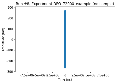
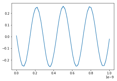
There seems to be something wrong with the plot_by_id method. Fixing this is beyond the scope of this PR. Below we show that the driver works properly

import matplotlib.pyplot as plt

plt.plot(
    tek.channel[i].waveform.trace_axis(),
    tek.channel[i].waveform.trace()
)

[<matplotlib.lines.Line2D at 0x2725fe33f60>]

Changing the waveform format

If we wish, we can change the way in which data is retrieved from the instrument, which can enhance the precision of the data and the speed to retrieval.

We do this through the ‘waveform’ module on the main driver (e.g. tek.waveform) as opposed to the ‘waveform’ module on a channel (e.g. tek.channel[0].waveform). We have this distinction because the waveform formatting parameters effect all waveform sources (e.g. channel 0 or channel 1)

tek.waveform.data_format()

'signed_integer'

# The available formats
tek.waveform.data_format.vals

<Enum: {'unsigned_integer', 'floating_point', 'signed_integer'}>

tek.waveform.is_big_endian()

True

tek.waveform.bytes_per_sample()

1

tek.waveform.bytes_per_sample.vals

<Enum: {8, 1, 2, 4}>

tek.waveform.is_binary()
# Setting is_binary to false will transfer data in ascii mode.

True

Trigger setup

The tek.trigger module is the ‘main’ trigger

tek.trigger.source()

'CH1'

tek.trigger.type()

'edge'

tek.trigger.edge_slope()

'fall'

tek.trigger.edge_slope("fall")

Delayed trigger

You can trigger with the Main trigger system alone or combine the Main trigger with the Delayed trigger to trigger on sequential events. When using sequential triggering, the Main trigger event arms the trigger system, and the Delayed trigger event triggers the instrument when the Delayed trigger conditions are met.

Main and Delayed triggers can (and typically do) have separate sources. The Delayed trigger condition is based on a time delay or a specified number of events.

See page75, Using Main and Delayed triggers of the manual

tek.delayed_trigger.source()

'CH1'

tek.delayed_trigger.type()

'edge'

Etc… The main and delayed triggers have the same parameters. However, the accepted values of these parameters might differ. Please see the above manual for details.

Measurements

The scope also has a measurement module

tek.measurement[0].source1("CH1")
tek.measurement[0].source2("CH2")
tek.measurement[1].source1("CH2")

channel = tek.measurement[0].source1()
value = tek.measurement[0].frequency()
unit = tek.measurement[0].frequency.unit

print(f"Frequency of signal at channel {channel}: {value:.2E} {unit}")

Frequency of signal at channel CH1: 9.96E+09 Hz

channel = tek.measurement[1].source1()
value = tek.measurement[1].frequency()
unit = tek.measurement[1].frequency.unit

print(f"Frequency of signal at channel {channel}: {value:.2E} {unit}")

Frequency of signal at channel CH2: 9.98E+09 Hz

channel = tek.measurement[0].source1()
value = tek.measurement[0].amplitude()
unit = tek.measurement[0].amplitude.unit

print(f"Amplitude of signal at channel {channel}: {value:.2E} {unit}")

Amplitude of signal at channel CH1: 2.84E-01 V

channel = tek.measurement[1].source1()
value = tek.measurement[1].amplitude()
unit = tek.measurement[1].amplitude.unit

print(f"Amplitude of signal at channel {channel}: {value:.2E} {unit}")

Amplitude of signal at channel CH2: 1.88E-01 V

channel1 = tek.measurement[0].source1()
channel2 = tek.measurement[0].source2()
value = tek.measurement[0].phase()
unit = tek.measurement[0].phase.unit

print(f"Phase of signal at channel {channel1} wrt channel {channel2}: {value} {unit}")

Phase of signal at channel CH1 wrt channel CH2: 25.50738557245 °

Here are all the availble measurements

from pprint import pprint

print_string = ", ".join([i[0] for i in TektronixDPOMeasurement.measurements])
pprint(print_string)

('amplitude, area, burst, carea, cmean, crms, delay, distduty, extinctdb, '
 'extinctpct, extinctratio, eyeheight, eyewidth, fall, frequency, high, hits, '
 'low, maximum, mean, median, minimum, ncross, nduty, novershoot, nwidth, '
 'pbase, pcross, pctcross, pduty, peakhits, period, phase, pk2pk, pkpkjitter, '
 'pkpknoise, povershoot, ptop, pwidth, qfactor, rise, rms, rmsjitter, '
 'rmsnoise, sigma1, sigma2, sigma3, sixsigmajit, snratio, stddev, undefined, '
 'waveforms')

Measurement statistics

We can measure basic measurement statistics

channel = tek.measurement[0].source1()
value = tek.measurement[0].amplitude.mean()
unit = tek.measurement[0].amplitude.unit

print(f"The mean amplitude of signal at channel {channel}: {value} {unit}")

The mean amplitude of signal at channel CH2: 0.284 V

We can do the same with all the measurement which are supported by the instrument. The following statistics are available: mean, max, min, stdev

Statistics control

A seperate module controls statistics gathring: tek.statistics. For instance, The oscilloscope gathers statistics over a set of measurement values which are stored in a buffer. We can reset this buffer like so…

tek.statistics.reset()

The following parameters are available for staistics control:

1. mode: This command controls the operation and display of measurement statistics and accepts the following arguments: OFF turns off all measurements. This is the default value. ALL turns on statistics and displays all statistics for each measurement. VALUEMean turns on statistics and displays the value and the mean (μ) of each measurement. MINMax turns on statistics and displays the min and max of each measurement. MEANSTDdev turns on statistics and displays the mean and standard deviation of each measurement.

2. time_constant: This command sets or queries the time constant for mean and standard deviation statistical accumulations

Future work

The DPO7200xx scopes have support for mathematical operations. An example of a math operation is a spectral analysis. Although the current QCoDeS driver does not (fully) support these operations, the way the driver code has been factored should make it simple to add support if future need arrises.

An example: we can manually add a spectrum analysis by selecting “math” -> “advanced spectral” from the oscilloscope menu in the front display of the instrument. After manual creation, we can retrieve spectral data with the driver as follows:

from qcodes.instrument_drivers.tektronix.DPO7200xx import TekronixDPOWaveform

math_channel = TekronixDPOWaveform(tek, "math", "MATH1")

meas = Measurement(exp=experiment)
meas.register_parameter(math_channel.trace)

with meas.run() as datasaver:

    datasaver.add_result(
        (math_channel.trace_axis, math_channel.trace_axis()),
        (math_channel.trace, math_channel.trace())
    )

    dataid = datasaver.run_id

plot_by_id(dataid)

Starting experimental run with id: 9

([<matplotlib.axes._subplots.AxesSubplot at 0x2725fa022b0>], [None])

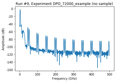
In order to fully support math operations and spectral analysis, we need code to add a math function through the QCoDeS driver, rather than manually. Additionally, we need to be able to adjust the frequency ranges and possibly other relevant parameters.

As always, contributions are more then welcome! :-)