This page was generated from
docs/examples/driver_examples/Qcodes example with Keithley 2600.ipynb.
Interactive online version:
![]() .
.
QCoDeS Example with with Keithley 2600 series
[ ]:
import qcodes as qc
from qcodes.dataset import (
    LinSweep,
    do0d,
    do1d,
    initialise_database,
    new_experiment,
    plot_dataset,
)
from qcodes.instrument_drivers.Keithley import Keithley2614B
[2]:
# Create a station to hold all the instruments

station = qc.Station()

# instantiate the Keithley and add it to the station

keith = Keithley2614B("keithley", "USB0::0x05E6::0x2614::4305420::INSTR")
station.add_component(keith)
Connected to: Keithley Instruments Inc. 2614B (serial:4305420, firmware:3.2.2) in 0.77s
[2]:
'keithley'
The Keithley 2600 has two channels, here called smua and smub in agreement with the instrument manual.
The two channels are basically two separate instruments with different integration times (nplc), operation modes (mode) etc.
[3]:
# Get an overview of the settings
#
# You will notice that the two channels have identical parameters but
# potentially different values for them
#
keith.print_readable_snapshot()
keithley:
        parameter      value
--------------------------------------------------------------------------------
IDN             :       {'vendor': 'Keithley Instruments Inc.', 'model': '2614B', '...
display_settext :       None
timeout         :       5 (s)
keithley_smua:
        parameter                  value
--------------------------------------------------------------------------------
curr                        :   8.7023e-07 (A)
fastsweep                   :   Not available
limiti                      :   0.1 (A)
limitv                      :   20 (V)
linefreq                    :   50 (Hz)
measure_autorange_i_enabled :   False
measure_autorange_v_enabled :   True
measurerange_i              :   0.1 (A)
measurerange_v              :   200 (V)
mode                        :   current
nplc                        :   0.05
output                      :   True
res                         :   2.2985e+07 (Ohm)
source_autorange_i_enabled  :   True
source_autorange_v_enabled  :   False
sourcerange_i               :   0.1 (A)
sourcerange_v               :   20 (V)
time_axis                   :   Not available (s)
timetrace                   :   Not available (A)
timetrace_dt                :   0.001 (s)
timetrace_mode              :   current
timetrace_npts              :   500
volt                        :   20.002 (V)
keithley_smub:
        parameter                  value
--------------------------------------------------------------------------------
curr                        :   -1.8239e-12 (A)
fastsweep                   :   Not available
limiti                      :   0.1 (A)
limitv                      :   20 (V)
linefreq                    :   50 (Hz)
measure_autorange_i_enabled :   True
measure_autorange_v_enabled :   True
measurerange_i              :   1e-07 (A)
measurerange_v              :   0.2 (V)
mode                        :   voltage
nplc                        :   1
output                      :   False
res                         :   3.5934e+07 (Ohm)
source_autorange_i_enabled  :   True
source_autorange_v_enabled  :   True
sourcerange_i               :   1e-07 (A)
sourcerange_v               :   0.2 (V)
time_axis                   :   Not available (s)
timetrace                   :   Not available (A)
timetrace_dt                :   0.001 (s)
timetrace_mode              :   current
timetrace_npts              :   500
volt                        :   -6.3276e-05 (V)
Basic operation
Each channel operates in either voltage or current mode. The mode controls the source behaviour of the instrument, i.e. voltage mode corresponds to an amp-meter (voltage source, current meter) and vice versa.
[4]:
# Let's set up a single-shot current measurement
# on channel a

keith.smua.mode("voltage")
keith.smua.nplc(
    0.05
)  # 0.05 Power Line Cycles per measurement. At 50 Hz, this corresponds to 1 ms
keith.smua.sourcerange_v(20)
keith.smua.measurerange_i(0.1)

keith.smua.volt(1)  # set the source to output 1 V
keith.smua.output("on")  # turn output on
curr = keith.smua.curr()
keith.smua.output("off")

print(f"Measured one current value: {curr} A")
Measured one current value: -3.40939e-06 A
Four-probe measurement
Enabling four-probe measurements is simple.
[ ]:
# Select channel to work with
smub = keith.smub

# Set up for four-probe measurement
smub.mode("current")  # Source current, measure voltage
smub.nplc(1.0)
smub.limitv(20)
smub.source_autorange_i_enabled(True)
smub.measure_autorange_v_enabled(True)

# Set sense mode
smub.four_wire_measurement(True)

# Make sure output is enabled
smub.output(True)

# Sweep parameters
i_start = 0  # A
i_stop = 0.1e-6  # A (0.1 µA)
n_points = 101
settle_delay = 0.001

# Take measurements
data, _, _ = do1d(smub.curr, i_start, i_stop, n_points, settle_delay, smub.volt)

# Set params to safe values
smub.curr(0)
smub.output(False)

plot_dataset(data)
Fast IV or VI curves
Onboard the Keithley 2600 sits a small computer that can interpret Lua scripts. This can be used to make fast IV- or VI-curves and is supported by the QCoDeS driver. To make IV- or VI-curves the driver has the ParameterWithSetpoints fastsweep, which has 3 modes: ‘IV’, ‘VI’ and ‘VIfourprobe’. The Modes ‘IV’ and ‘VI’are two probe measurements, while the mode ‘VIfourprobe’ makes a four probe measurement.
1D Fast Sweep
Let’s make a fast IV curve by sweeping the voltage from 1 V to 2 V in 500 steps. Create a LinSweep object and pass it to setup_fastsweep, then call do0d on fastsweep.
NOTE on LinSweep: LinSweep isn’t specifically required here. We just need a _LinSweepLike object to pass, which requires param, delay, and num_points attributes and a get_setpoints() method.
NOTE on fastsweep: Users may decide which channel the current/voltage is measured from during a fastsweep. It is usually expected to measure the channel that is being swept (which is the default behavior), but in cases where your measurement requires you to collect data from some other terminal (e.g., if you are sweeping voltage on terminal A and want to measure current on terminal B), you can set measure_inner_channel=False in setup_fastsweep.
[ ]:
# Configure a 1D fastsweep using LinSweep
fast_sweep_1d = LinSweep(keith.smua.volt, 1, 2, 500)
keith.smua.setup_fastsweep(fast_sweep_1d, mode="IV", measure_inner_channel=True)

# Perform the measurement
ds, _, _ = do0d(keith.smua.fastsweep)
plot_dataset(ds)
2D Fast Sweep
For 2D sweeps, provide both inner and outer LinSweep objects. The inner sweep runs to completion for each step of the outer sweep. The measurement is performed on the inner channel (the one from the first LinSweep).
Here we sweep smua.volt (inner/fast axis) while stepping smub.volt (outer/slow axis):
[ ]:
# Configure a 2D fastsweep: inner on smua, outer on smub
inner_sweep = LinSweep(keith.smua.volt, -1, 1, 100)  # inner (fast axis)
outer_sweep = LinSweep(keith.smub.volt, 0, 0.5, 20)  # outer (slow axis)

keith.smua.setup_fastsweep(inner_sweep, outer_sweep, mode="IV")

# Perform the measurement - call fastsweep on the inner channel (smua)
ds, _, _ = do0d(keith.smua.fastsweep)
plot_dataset(ds)
Time Trace
We can measure current or voltage as a function of time, as well. Let us consider the case in which we would like to have the time trace of current. We, then, first set our trace mode accordingly
[9]:
keith.smua.timetrace_mode("current")
The latter should not be confused with the channel mode. Next, we register our parameter
[10]:
timemeas = qc.Measurement()
timemeas.register_parameter(keith.smua.timetrace)
[10]:
<qcodes.dataset.measurements.Measurement at 0x1cb25ae9eb0>
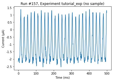
The total time interval is returned by time_axis method in accordance with the integration time dt and the total number of points npts with default values of 1 ms and 500, respectively. Specifically, the time trace will be obtained for an interval of [0, dt*npts]. Thus, for the default values, we shall have a time trace of current for 500 ms calculated at 500 steps.
[11]:
keith.smua.timetrace_dt()
[11]:
0.001
[12]:
keith.smua.timetrace_npts()
[12]:
500
[13]:
initialise_database()
new_experiment(name="tutorial_exp", sample_name="no sample")

with timemeas.run() as datasaver:
    somenumbers = keith.smua.timetrace.get()
    datasaver.add_result(
        (keith.smua.timetrace, somenumbers),
        (keith.smua.time_axis, keith.smua.time_axis.get()),
    )

data = datasaver.dataset
plot_dataset(data)
Starting experimental run with id: 157.
[13]:
([<AxesSubplot:title={'center':'Run #157, Experiment tutorial_exp (no sample)'}, xlabel='Time (ms)', ylabel='Current (μA)'>],
 [None])

Let us get another trace for 2ms integration time with 600 steps
[14]:
keith.smua.timetrace_dt(0.002)
[15]:
keith.smua.timetrace_npts(600)
[16]:
with timemeas.run() as datasaver:
    somenumbers = keith.smua.timetrace.get()
    datasaver.add_result(
        (keith.smua.timetrace, somenumbers),
        (keith.smua.time_axis, keith.smua.time_axis.get()),
    )

data = datasaver.dataset
plot_dataset(data)
Starting experimental run with id: 158.
[16]:
([<AxesSubplot:title={'center':'Run #158, Experiment tutorial_exp (no sample)'}, xlabel='Time (s)', ylabel='Current (μA)'>],
 [None])
Similarly, we can get the time trace for voltage via changing the mode
[18]:
keith.smua.timetrace_mode("voltage")
In this case, one should re-register the time trace parameter to have the correct units and labels.
Recalibration
Sometimes it happens that Keithley SMU measures a different value from what was assigned as the setpoint; e.g. when setting the voltage to -2 mV, the SMU would measure an output of -1.85 mV. This likely calls for recalibration of the Keithley SMU against e.g. a calibrated DMM. After this recalibration the measured value matches the setpoint.
Below is a description of using a calibration routine that is based off the information from the instrument manual about performing the calibration.
To run this routine, connect the Keithley SMU HI voltage output to the DMM voltage HI input, and the SMU LO output to the DMM voltage LO input (note that this is a different setup as indicated in the Keithley manual).
[ ]:
# %% Imports

# The calibration functions and utils
from qcodes.calibrations.keithley import (
    calibrate_keithley_smu_v,
    calibrate_keithley_smu_v_single,
    save_calibration,
    setup_dmm,
)

# QCoDeS functions for running a measurement
from qcodes.dataset import do1d, load_or_create_experiment

# Keithley SMU driver
from qcodes.instrument_drivers.Keithley import Keithley2614B

# Keysight DMM driver
from qcodes.instrument_drivers.Keysight import Keysight34470A

# %% Load the SMU instrument
smu = Keithley2614B("smu", "USB0::0x05E6::0x2614::4347170::INSTR")

# %% Load DMM instrument
dmm = Keysight34470A("dmm", "TCPIP0::10.164.54.211::inst0::INSTR")

# %% Calibrate both channels
calibrate_keithley_smu_v(smu, dmm)
for smun in smu.channels:
    smun.volt(0)

# %% Calibrate single channel in specific range, e.g. SMU A
smun = smu.smua  # e.g. SMU A

setup_dmm(dmm)
dmm.range(1.0)
calibrate_keithley_smu_v_single(smu, smun.short_name, dmm.volt, "200e-3")
smun.volt(0)

# %% Check calibration by measuring voltage with DMM while sweeping with SMU
smun = smu.smua  # e.g. SMU A

smun.sourcerange_v(200e-3)
smun.measurerange_v(200e-3)
smun.volt(0)
smun.output("on")

dmm.aperture_time(0.1)
dmm.range(1)
dmm.autozero("OFF")
dmm.autorange("OFF")

load_or_create_experiment(
    "MeasurementSetupDebug", "no_sample", load_last_duplicate=True
)

do1d(
    smun.volt,
    -0.1e-3,
    0.1e-3,
    101,
    0.3,
    dmm.volt,
    smun.curr,
    measurement_name=f"{smun.full_name} calibration check",
)

smun.volt(0)
smun.output("off")

# %% Save calibrations
save_calibration(smu)