This page was generated from
docs/examples/DataSet/Offline plotting with complex data.ipynb.
Interactive online version:
![]() .
.
Offline plotting with complex data
This notebook is a collection of plotting examples using the plot_dataset function and complex data. We cover the cases where the dependent (measured) parameter is complex, and the case where the independent parameter is complex.
The behavior of the plot_dataset with respect to compex-valued parameters is as follows: one complex-valued parameter is converted into two real-valued parameters.
We start by initialising our database and creating an experiment.
[1]:
%matplotlib inline
from pathlib import Path

import numpy as np

from qcodes.dataset import (
    Measurement,
    initialise_or_create_database_at,
    load_or_create_experiment,
    plot_dataset,
)
[2]:
initialise_or_create_database_at(
    Path.cwd().parent / "example_output" / "offline_plotting_example_complex.db"
)
exp = load_or_create_experiment("offline_plotting_complex_numbers", "")
Case A: a complex number as a function of a real number
Now, we are ready to perform a measurement. To this end, let us register our custom parameters.
[3]:
meas_A = Measurement(exp)
meas_A.register_custom_parameter(
    name="freqs", label="Frequency", unit="Hz", paramtype="numeric"
)
meas_A.register_custom_parameter(
    name="iandq",
    label="Signal I and Q",
    unit="V^2/Hz",
    paramtype="complex",
    setpoints=["freqs"],
)
[3]:
<qcodes.dataset.measurements.Measurement at 0x7fc81f910d40>
[4]:
N = 1000
freqs = np.linspace(0, 1e6, N)
signal = np.cos(2 * np.pi * 1e-6 * freqs) + 1j * np.sin(2 * np.pi * 1e-6 * freqs)

with meas_A.run() as datasaver:
    datasaver.add_result(("freqs", freqs), ("iandq", signal))

ds = datasaver.dataset
Starting experimental run with id: 1.
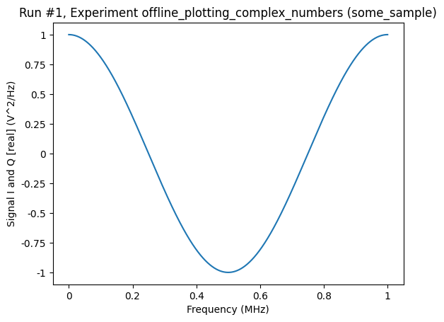
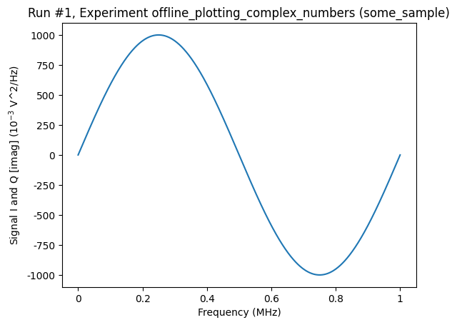
When visualising the data, the plot_dataset will turn the complex signal parameter into to real parameters. The plot_dataset function can do this “transformation” in one of two ways: either casting the amplitudes of the real and imaginary parts or calculating the magnitude and phase. By default, the plot_dataset uses the former.
[5]:
axs, cbs = plot_dataset(ds)
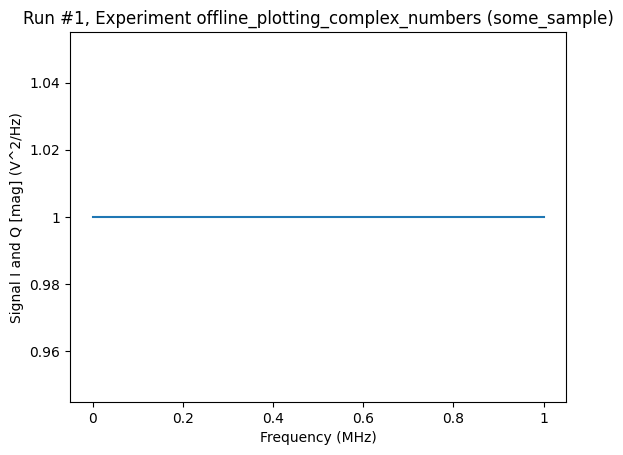
[6]:
axs, cbs = plot_dataset(ds, complex_plot_type="mag_and_phase")

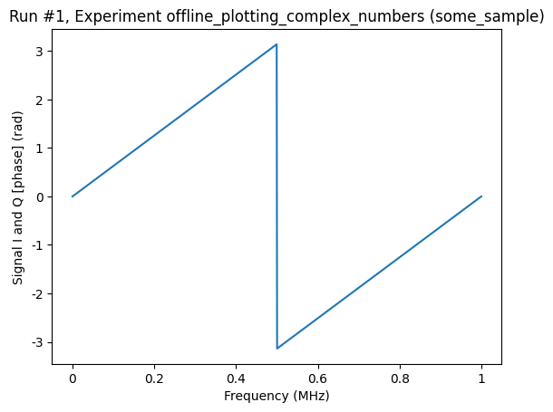
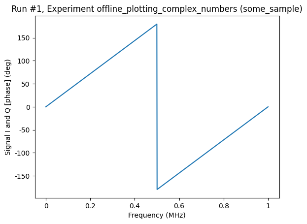
Note that the phase can be visualized either in degrees or in radians. The keyword argument complex_plot_phase of the plot_dataset function controls this behaviour. The default is radians.
[7]:
axs, cbs = plot_dataset(
    ds, complex_plot_type="mag_and_phase", complex_plot_phase="degrees"
)
Case B: a complex number as a function of two real numbers
[8]:
meas_B = Measurement(exp)
meas_B.register_custom_parameter(
    name="freqs", label="Frequency", unit="Hz", paramtype="numeric"
)
meas_B.register_custom_parameter(
    name="magfield", label="Magnetic field", unit="T", paramtype="numeric"
)
meas_B.register_custom_parameter(
    name="iandq",
    label="Signal I and Q",
    unit="V^2/Hz",
    paramtype="complex",
    setpoints=["freqs", "magfield"],
)
[8]:
<qcodes.dataset.measurements.Measurement at 0x7fc81c420f50>
[9]:
N = 250
M = 20
freqs = np.linspace(0, 1e6, N)
fields = np.linspace(0, 2, M)

with meas_B.run() as datasaver:
    for field in fields:
        phis = 2 * np.pi * field * 1e-6 * freqs
        signal = np.cos(phis) + 1j * np.sin(phis)
        datasaver.add_result(("freqs", freqs), ("iandq", signal), ("magfield", field))

run_B_id = datasaver.run_id
ds2 = datasaver.dataset
Starting experimental run with id: 2.
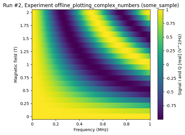
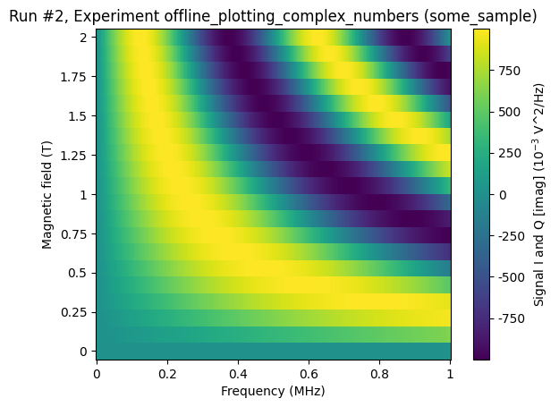
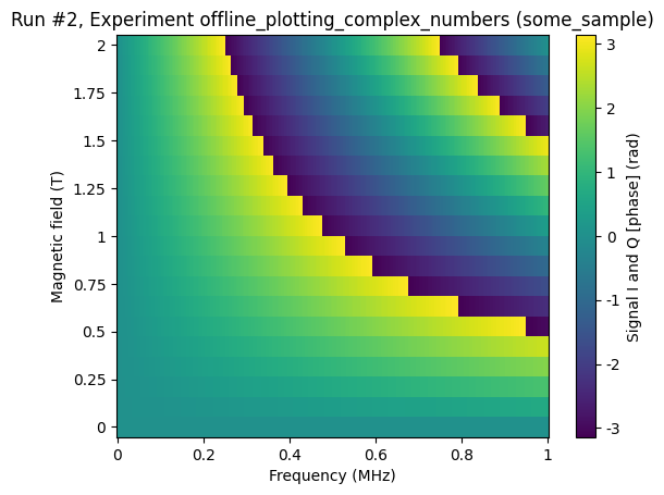
When visualising this run, we get two plots just as in the previous case. This time, however, the plots are heatmaps and not line plots.
[10]:
axs, cbs = plot_dataset(ds2, complex_plot_type="real_and_imag")
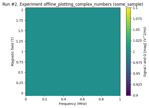
[11]:
axs, cbs = plot_dataset(ds2, complex_plot_type="mag_and_phase")
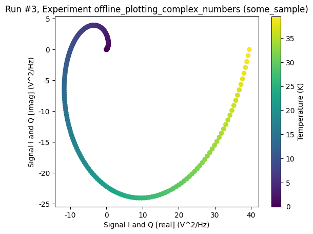
Case C: a real number as a function of a complex number
As expected, the single complex setpoint parameter is turned into two real-valued setpoint parameters.
[12]:
meas_C = Measurement(exp)
meas_C.register_custom_parameter(
    name="iandq", label="Signal I and Q", unit="V^2/Hz", paramtype="complex"
)
meas_C.register_custom_parameter(
    name="temp", label="Temperature", unit="K", paramtype="numeric", setpoints=["iandq"]
)
[12]:
<qcodes.dataset.measurements.Measurement at 0x7fc81c495760>
[13]:
N = 250
phis = 2 * np.pi * np.linspace(1e-9, 1, N)
signal = phis**2 * (np.cos(phis) + 1j * np.sin(phis))
heat = np.abs(signal)

with meas_C.run() as datasaver:
    datasaver.add_result(("iandq", signal), ("temp", heat))

run_C_id = datasaver.run_id
ds3 = datasaver.dataset
Starting experimental run with id: 3.
[14]:
axs, cbs = plot_dataset(ds3)
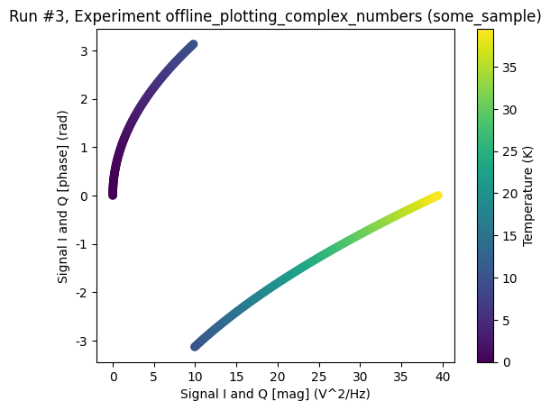
[15]:
axs, cbs = plot_dataset(ds3, complex_plot_type="mag_and_phase")
[ ]: