Methods for Multiscale Comparative Connectomics

This demo shows you how to use methods in graspologic to analyze patterns in brain connectivity in connectomics datasets. We specifically demonstrate methods for identifying differences in edges and vertices across subjects.

import matplotlib.pyplot as plt
import numpy as np
import pandas as pd
import seaborn as sns
import warnings
pd.options.mode.chained_assignment = None
%matplotlib inline

Load the Duke mouse brain dataset

Dataset of 32 mouse connectomes derived from whole-brain diffusion magnetic resonance imaging of four distinct mouse genotypes: BTBR T+ Itpr3tf/J (BTBR), C57BL/6J(B6), CAST/EiJ (CAST), and DBA/2J (DBA2). For each strain, connectomes were generated from eight age-matched mice (N = 8 per strain), with a sex distribution of four males and four females. Each connectome was parcellated using asymmetric Waxholm Space, yielding a vertex set with a total of 332 regions of interest (ROIs) symmetrically distributed across the left and right hemispheres. Within a given hemisphere, there are seven superstructures consisting up multiple ROIs, resulting in a total of 14 distinct communities in each connectome.

from graspologic.datasets import load_mice

# Load the full mouse dataset
mice = load_mice()

# Stack all adjacency matrices in a 3D numpy array
graphs = np.array(mice.graphs)

# Get sample parameters
n_subjects = mice.meta["n_subjects"]
n_vertices = mice.meta["n_vertices"]

# Split the set of graphs by genotype
btbr = graphs[mice.labels == "BTBR"]
b6 = graphs[mice.labels == "B6"]
cast = graphs[mice.labels == "CAST"]
dba2 = graphs[mice.labels == "DBA2"]

connectomes = [btbr, b6, cast, dba2]

Identifying Signal Edges

The simplest approach for comparing connectomes is to treat them as a bag of edges without considering interactions between the edges. Serially performing univariate statistical analyses at each edge enables the discovery of signal edges whose neurological connectivity differs across categorical or dimensional phenotypes. Here, we demonstrate the possibility of using Distance Correlation (Dcorr), a nonparametric universally consistent test, to detect changes in edges.

In this model, we assume that each edge in the connectome is independently and identically sampled from some distribution \(F_i\), where \(i\) represents the group to which the given connectome belongs. In this setting the groups are the mouse genotypes. Dcorr allows us to test the following hypothesis:

\begin{align*} H_0:\ &F_1 = F_2 = \ldots F_k \\ H_A:\ &\exists \ j \neq j' \text{ s.t. } F_j \neq F_{j'} \end{align*}

from hyppo.ksample import KSample

Since the connectomes in this dataset are undirected, we only need to do edge comparisons on the upper triangle of the adjacency matrices.

# Make iterator for traversing the upper triangle of the connectome
indices = zip(*np.triu_indices(n_vertices, 1))

edge_pvals = []

for roi_i, roi_j in indices:

    # Get the (i,j)-th edge for each connectome
    samples = [genotype[:, roi_i, roi_j] for genotype in connectomes]

    # Calculate the p-value for the (i,j)-th edge
    try:
        statistic, pvalue = KSample("Dcorr").test(*samples, reps=10000, workers=-1)
    except ValueError:
        # A ValueError is thrown when any of the samples have equal edge
        # weights (i.e. one of the inputs has 0 variance)
        statistic = np.nan
        pvalue = 1

    edge_pvals.append([roi_i, roi_j, statistic, pvalue])

Connectomes are a high-dimensional dataype. Thus, statistical tests on components of the connectome (e.g. edge and vertices) results in multiple comparisons. We recommend correcting for multiple comparisons using the Holm-Bonferroni (HB) corection.

The algorithm is described below: 1. Sort the p-values from lowest-to-highest \(P_1, P_2, \dots, P_n\), where \(n\) is the number of tests 2. Correct the p-value as \(P_1(n), P_2(n-1), \dots, P_n(1)\) 3. If any corrected p-value is \(>1\), replace with \(1\) 4. If the corrected p-value is less than a significance level \(\alpha\), reject

# Convert the nested list to a dataframe
edge_pvals = pd.DataFrame(edge_pvals, columns=["ROI_1", "ROI_2", "stat", "pval"])

# Correct p-values using the Holm-Bonferroni correction
edge_pvals.sort_values(by="pval", inplace=True, ignore_index=True)
pval_rank = edge_pvals["pval"].rank(ascending=False, method="max")
edge_pvals["holm_pval"] = edge_pvals["pval"].multiply(pval_rank)
edge_pvals["holm_pval"] = edge_pvals["holm_pval"].apply(
    lambda pval: 1 if pval > 1 else pval
)

# Test for significance using alpha=0.05
alpha = 0.05
edge_pvals["significant"] = (edge_pvals["holm_pval"] < alpha)

# Get the top 10 strongest signal edges
edge_pvals_top = edge_pvals.head(10)

# Replace ROI indices with actual names
def lookup_roi_name(index):
    hemisphere = "R" if index // 166 else "L"
    index = index % 166
    roi_name = mice.atlas.query(f"ROI == {index+1}")["Structure"].item()
    return f"{roi_name} ({hemisphere})"

edge_pvals_top["ROI_1"] = edge_pvals_top["ROI_1"].apply(lookup_roi_name)
edge_pvals_top["ROI_2"] = edge_pvals_top["ROI_2"].apply(lookup_roi_name)

edge_pvals_top.head()

	ROI_1	ROI_2	stat	pval	holm_pval	significant
0	Corpus_Callosum (L)	Striatum (R)	0.717036	9.911903e-07	0.054462	False
1	Corpus_Callosum (L)	Internal_Capsule (R)	0.699473	1.327371e-06	0.072932	False
2	Corpus_Callosum (L)	Reticular_Nucleus_of_Thalamus (R)	0.698197	1.355858e-06	0.074496	False
3	Corpus_Callosum (L)	Zona_Incerta (R)	0.685735	1.668308e-06	0.091662	False
4	Septum (R)	Corpus_Callosum (R)	0.670809	2.139082e-06	0.117525	False

Note that none of the edges achieve significance at \(\alpha=0.05\) following Holm-Bonferroni correction. We might expect this, given that we are correcting for \(N=54,946\) tests. Instead of the magnitude, the ranking of the p-values can be used to determine signal edges.

Identifying Signal Vertices

A sample of connectomes can be jointly embedded in a low-dimensional Euclidean space using the omnibus embedding (omni). A host of machine learning tasks can be accomplished with this joint embedded representation of the connectome, such as clustering or classification of vertices. Here, we use the embedding to formulate a statistical test that can be used to identify vertices that are strongly associated with given phenotypes. According to a Central Limit Theorem for omni, these latent positions are universally consistent and asymptotically normal.

from graspologic.embed import OmnibusEmbed
from graspologic.plot import pairplot

# Jointly embed graphs using omnibus embedding
embedder = OmnibusEmbed()
omni_embedding = embedder.fit_transform(graphs)
print(omni_embedding.shape)

(32, 332, 5)

For each of the 32 mice, omni embeds each vertex in the connectome to a latent position vector \(x_i \in \mathbb{R}^5\). We test for differences in the distribution of vertex latent positions using the MGC independence test implemented in hyppo. This test essentially acts as a nonparametric MANOVA test.

with warnings.catch_warnings():
    warnings.filterwarnings("ignore", module="hyppo")
    warnings.filterwarnings("ignore", category=RuntimeWarning)
    vertex_pvals = []

    for vertex_i in range(n_vertices):

    # Get the embedding of the i-th vertex for
        samples = [
            omni_embedding[mice.labels==genotype, vertex_i, :]
            for genotype in np.unique(mice.labels)
        ]

    # Calculate the p-value for the i-th vertex
        statistic, pvalue, _ = KSample("MGC").test(
            *samples, reps=250, workers=-1
        )
        vertex_pvals.append([vertex_i, statistic, pvalue])

Important: When running on data, make sure reps \(\geq \frac{|V|}{\alpha}\) where \(|V|\) is the cardinality of the vertex set and \(\alpha\) is the significance level for your test. Again, this has to do with p-value correction: because MGC is a permutation test, you need many replications to ensure accurate computation of the p-value. Because this notebook is primarily for demonstration purposes, we use a small value of reps=250. For this dataset, a more appropriate number of permutations would be around \(10^6\).

# Convert the nested list to a dataframe
vertex_pvals = pd.DataFrame(vertex_pvals, columns=["ROI", "stat", "pval"])

# Correct p-values using the Holm-Bonferroni correction
vertex_pvals.sort_values(by="pval", inplace=True, ignore_index=True)
pval_rank = vertex_pvals["pval"].rank(ascending=False, method="max")
vertex_pvals["holm_pval"] = vertex_pvals["pval"].multiply(pval_rank)
vertex_pvals["holm_pval"] = vertex_pvals["holm_pval"].apply(
    lambda pval: 1 if pval > 1 else pval
)

# Test for significance using alpha=0.05
alpha = 0.05
vertex_pvals["significant"] = (vertex_pvals["holm_pval"] < alpha)

# Get the top 10 strongest signal edges
vertex_pvals_top = vertex_pvals.head(10)

# Replace ROI indices with actual names
vertex_pvals_top["ROI"] = vertex_pvals_top["ROI"].apply(lookup_roi_name)

vertex_pvals_top.head()

	ROI	stat	pval	holm_pval	significant
0	Cingulate_Cortex_Area_24a (L)	0.754901	0.003984	1.0	False
1	Hypothalamus (R)	0.664767	0.003984	1.0	False
2	Amygdalopiriform_Transition_Area (R)	0.526762	0.003984	1.0	False
3	Piriform_Cortex (R)	0.603432	0.003984	1.0	False
4	Presubiculum (R)	0.292116	0.003984	1.0	False

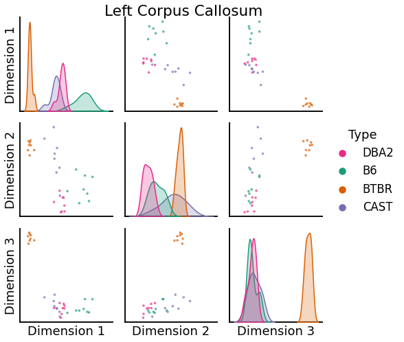
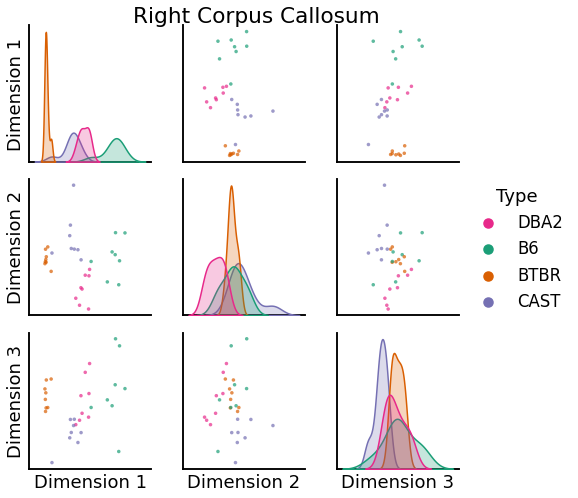
We can use pairplots to visualize the embeddings of specific vertices. Below are pairsplots of the corpus callosum from the left and right hemispheres.

left = pairplot(
    omni_embedding[:, 121 - 1, :3],
    mice.labels,
    palette=["#e7298a", "#1b9e77", "#d95f02", "#7570b3"],
    title="Left Corpus Callosum"
)

right = pairplot(
    omni_embedding[:, 121 + 166 - 1, :3],
    mice.labels,
    palette=["#e7298a", "#1b9e77", "#d95f02", "#7570b3"],
    title="Right Corpus Callosum",
)

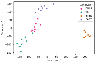
Whole-brain Comparisons

We can use the results of the omnibus embedding to perform whole-brain comparisons across subjects from different phenotypes.

from graspologic.embed import ClassicalMDS
from graspologic.plot import heatmap

Two-dimensional representations of each connectome were obtained by using Classical Multidimensional Scaling (cmds) to reduce the dimensionality of the embeddings obtained by omni.

# Further reduce embedding dimensionality using cMDS
cmds = ClassicalMDS(2)
cmds_embedding = cmds.fit_transform(omni_embedding)
cmds_embedding = pd.DataFrame(cmds_embedding, columns=["Dimension 1", "Dimension 2"])
cmds_embedding["Genotype"] = mice.labels

# Embedding with BTBR
sns.scatterplot(
    x="Dimension 1",
    y="Dimension 2",
    hue="Genotype",
    data=cmds_embedding,
    palette=["#e7298a", "#1b9e77", "#d95f02", "#7570b3"],
)
plt.show()

# Find the dissimilarity between subjects' connectomes using the cMDS embedding
dis = cmds.dissimilarity_matrix_
scaled_dissimilarity = dis / np.max(dis)

heatmap(scaled_dissimilarity,
        context="paper",
        inner_hier_labels=mice.labels,)
plt.show()

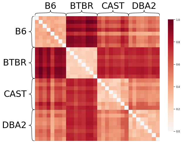
Notice that mice from the same genotype are most similar to each other, as expected.