Here the topics on the other pages will be applied in a straight-forward manner. As such, it omits a lot of the explanations behind the various concepts. If certain parts are confusing, consult the appropriate page on the topic.
(OPTIONAL). The guide assumes you follow these.Introduction
Requirements
-
Familiarity with basic AnyLogic concepts (reference: AnyLogic Help)
-
You have a Bonsai account setup (reference: Bonsai documentation for “how-to”)
-
Beginner-level familiarity with Inkling code (reference: Bonsai documentation for Inkling)
About the model
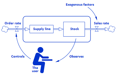
This simulation consists of a small system dynamics model that depicts a simple supply chain. Exogenous factors influence how quickly an inventory – referred to as “Stock” – depletes. The “game” component is that every 50 days, the model pauses itself, allowing you (as the user) to observe the stock level, set what the order rate should be, and resume the model again.
A diagram of this process (from the original model) can be seen below. Of relevance, but not shown in the image, is a parameter called “AcquisitionLag” whose value determines how many days it takes to receive the full order from the supply line to the stock on-hand.
Goal: Automate the decision-making process so that “the user” can be replaced with an AI.
The AI should be able to effectively control the order rate within the same bounds as the user can control (via the slider) - between 0 and 50 - and ideally the stock level should be between 1000-3000.
The base model does not impose an upper limit on how high the stock can be. Considering that the order rate can go up to 50 (per day), and the time between actions (50 days), this will result in a maximum change over one iteration to be 2500 additional stock (50*50). The range [1000-3000] is used, as it’s generally around this amount and uses nice round numbers. This is good enough, as this is a simple toy model.
0. Getting started
Prerequisite: Any edition of AnyLogic with the Bonsai Connector Library added to your environment.
-
Open the example model from Help > Models from ‘The Big Book of Simulation Modeling’ > System dynamics and dynamic systems > Stock Management Game.
-
Create a copy of it by right clicking the model’s name > Save As… > choosing a desired location.
1. Model Setup
To start adapting this model to one that is “RL-ready”, there are some facilitating additions to include.
1a. (OPTIONAL) Implement an automated control policy
In real-world models, the logic will be controlled by some heuristic-based logic rather than being entirely manual. To recreate this, we can add a function that, when called, will update the rate based on the current stock level using some heuristic.
-
Drag in a new function from the Agent palette to Main and call it “heuristicAction”.
-
In the body, write code such that if Stock is less than or equal to 1500, OrderRate increases by 10; else, if Stock is greater than or equal to 2000, it should decrease by 10. Additionally, use the built-in function limit to constrain OrderRate between 0 and 50. See the image below for an example implementation.
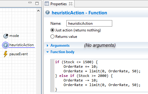
Implementation of step 1a (control policy)
A visual representation for how the heuristic behaviors can be seen in the image below. At each decision point (every 50 days), the order rate (in green) is updated based on the stock level (in blue). On the iterations where the stock value falls outside the range described in the logic (dotted lines), the order rate changes.
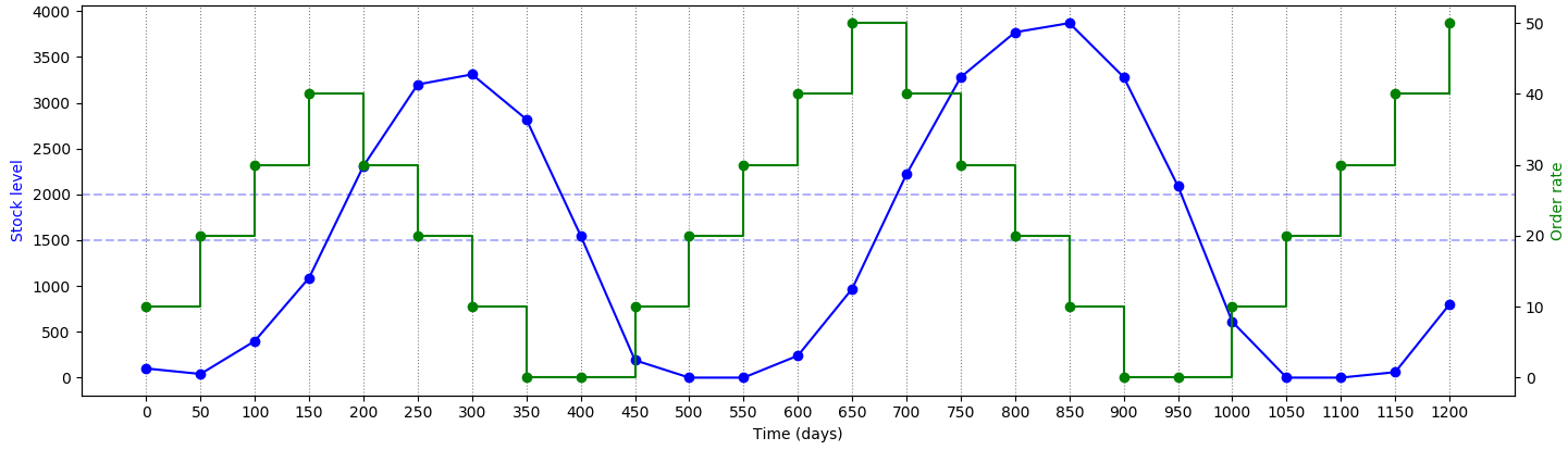
This specific policy was found in a similar way as simple inventory policies are optimized. Three temporary parameters were added to the model - representing the possible lower bound, upper bound, and step size. Two integer variables were also added as counters to keep track of when the stock was or was not within the bounds. An optimization was then executed that attempted to find parameter values that maximized the time in the range. All ranges were kept as discrete for simplicity. One run found the respective values of 1500, 2000, and 10 to be optimal. Afterwards, the parameters, variables, and experiment were deleted.
1b. (OPTIONAL) Adding the “mode” parameter
When the model encounters a decision point (to decide the next order rate) every 50 days, there are four different ways it can behave. Each has different logic associated with it. They are as follows:
-
Heuristic – update the rate automatically, using the implemented control policy
-
Interactive – the model pauses itself to let the user interact with it (as in the original model)
-
Brain training (either locally hosted or uploaded training) – the model queries the learning agent (the brain) for an action based on the current observation
-
Brain assessment (for testing a trained brain) – the model queries a trained, exported brain for an action at a specified HTTP endpoint
-
Drag in a new parameter from the Agent palette to Main – call it “mode”, set its type to int.
-
Update the Value Editor section by setting the control type field to ‘Radio Button’ and assigning the aforementioned labels and values.
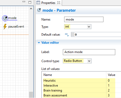
Implementation of 1b (the mode parameter)
Simulation experiment properties with the mode parameter added
2. Adding the RL Experiment
After going through the setup process, the first RL-related step is to add a new RL Experiment and determine what the Observation, Action, and Configuration should consist of.
-
Add a new RL Experiment by right clicking the model’s name in the Projects panel > New… > Experiment > Reinforcement Learning.
-
(OPTIONAL) Keep the default name (“RLExperiment”).
Using default name is recommended here, as subsequent steps call a specific function contained in the experiment’s Java class. If you choose a different name; you’ll just refer to that name instead.
2a. Observation section
The observation is what is passed to the brain at the start of each iteration (i.e., after a decision point is triggered). It contains fields which will be used by the brain to determine an action and may also be used as part of the training regimen to define terminal conditions or part of goal statements.
-
Fill out the data field table and assign the variables in the subsequent code area (code example shown in the image below):
-
In the table, add rows for three variables of type double: the current stock value (e.g., “stock_value”), the last order rate assigned (e.g., “last_order_rate”), and the current model time in days (e.g., “time_days”).
-
In the code area, assign the three variables based on the values inside the top-level agent (accessed via the “root” keyword).
-
Providing the stock value to the brain is the most basic piece of information to determine the new order rate.
Providing the last order rate (i.e., what was set in the last iteration) might give some useful context to the brain, serving as a very primitive form of memory.
Providing the current time allows you to optionally set time-based terminal criteria as part of your Bonsai training code.
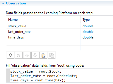
Observation section in the RL experiment
The variable name for time – “time_days” - includes the unit as a reminder when we are later in the Bonsai UI and might not remember the specific units that were used in the model.
The Observation section has a field called “Simulation run stop condition”. Bonsai requires us to define terminal conditions in its UI, so this should always be set to the Java keyword false.
2b. Action section
The action section is where you define the names of variables that the brain will choose values for, and where you apply those values within your model.
-
Fill out the data field table and write the code that will assign that value (code example shown in the image below):
-
In the table, add a row for the order rate (e.g., “order_rate”) and set its type as a double.
-
In the code area, update the OrderRate object inside the top-level agent (accessed via the keyword root) to the value of the order rate provided by the brain.
-
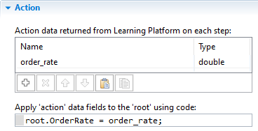
Action section in the RL experiment
2c. Configuration section
The configuration section is where you define and assign variables you will want to have the ability to change at the start of each training episode. These operate similar to simulation parameters.
-
Fill out the data field table and write the code that will assign the values (code example shown in the image below):
-
In the table, add a row for the number of days to lag order acquisition (e.g., “acquisition_lag_days”); set its type to int.
-
In the code area, update the AcquisitionLag parameter in the top-level agent (accessed via the root keyword) with the passed value. Additionally, hard code the mode parameter to be set to the value corresponding to the training mode.
-
Having a lag might better represent the delays present in real-world scenarios, but it also makes it harder for the brain to learn an effective policy. During training, we may wish to initially train the brain with easier scenarios – like instant acquisition (i.e., where lag is set to 1) – and incrementally increase the difficulty.
Critical: If you do not hard code the assigned value of mode, it will be assigned to whatever the “Default value” is set to in the parameter’s properties. Not having mode set to the correct value will affect the logic (which we’ll add in the next step) and cause problems with training (e.g., iterations never being triggered).
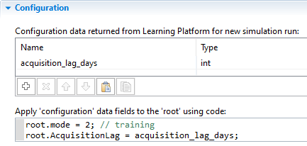
Configuration section in the RL experiment
If there’s any concern any input validation (e.g., invalid values being passed), you may wish to add code that handles for this. If this example, the value should never be below 1, so you could use AnyLogic’s built-in limitMin function to ensure this is always the case (e.g., limitMin(1, acquisition_lag_days)).
2d. Other common sections
As with other AnyLogic experiments, there are a few common sections that you should review.
- In the model time section, set stop mode to “Never” (stop conditions must be defined in Bonsai)
- In the randomness section, select the option for “Random seed”
Setting this to a fixed seed would cause the brain to learn from the same demand fluctuations across every episode. This wouldn’t be ideal if we want the Brain to be flexible in a variety of situations, as it wouldn’t otherwise have had the experience to learn how to effectively deal with unexpected scenarios it had not previously seen before.
3. Adding the Iteration Trigger
This section adds the logic and code related to triggering iterations (i.e., the point in simulation time when we want to request an action from the brain).
The original model had an Event object called “pauseEvent” which was used as a decision-making point. Specifically, it called the pauseSimulation function, allowing the user to take an action.
We’ll make a few changes to the event to adapt it to our needs (the numbering corresponding to the labels in the image below):
-
(OPTIONAL) Change name of “pauseEvent” to “actionEvent”
Renaming the object is recommended, as the Action code of this object will be updated to do more than simply pausing.
-
Add some if/else-if statements to execute code appropriate to the value of the mode parameter (code shown in the image below): Mode 0 will call the heuristicAction function; mode 1 will call the pauseSimulation function (as in the original model); modes 2 and 3 will call the takeAction function within the RLExperiment class.
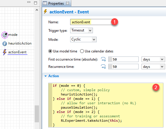
The updated event object in this model
The model logic is now updated to react based on the value of the mode parameter. Here is what you should expect if you try to run the model in the different modes:
-
When the event fires (every 50 days), if the value of Stock is below 1500 or above 2000, you should see a change in the “Order Rate” graph.
The slider will not automatically update (this has no effect on the model logic). If it’s desired to add this feature, you can manually update its current value by including the following line of code at the end of the “heuristicAction” function: slider.setValue(OrderRate);
-
When the event fires, the model should pause itself and you can control the slider manually. Pressing play will resume the simulation. This is equivalent to how the original model operated.
-
When the Event fires, the model will throw an error with a message like “The model should define the learning agent interface”.
- Same as Mode 2.
4. (OPTIONAL) Adding the Bonsai Connector
To get setup in Bonsai with this model, we will first perform locally hosted training. In doing so, you will train a brain in Bonsai’s webapp while connected to the model running on your local machine. While you can only train with one instance of your model at a time, it’s useful for being able to quickly test the connection before uploading the model for scaled training.
To facilitate the communication between the local AnyLogic model and Bonsai, the Bonsai Connector object is necessary.
- Drag in a new instance of the Connector from the “Bonsai Library” tab in your Palette panel. In its properties, perform the following:
-
Change the input option for “Enable connector” by clicking on the equal sign (“=”) and selecting “Static Value”. Delete where it says true and replace it with the code: mode >= 2
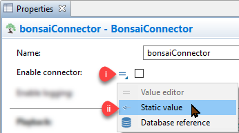

This condition will evaluate once, after the model starts, and cause the Connector to only enable if the value of the mode parameter is 2 or higher (corresponding to training or assessment).
Note: When the Bonsai Connector is enabled, it will take complete control of the model on startup (as the training regimen you setup in later sections will determine how the model is controlled). -
Repeat step 1, but for the “Playback” setting and in the conditional statement, replace where it says true with the code: mode == 3
This makes it so that the Playback feature will only be enabled if the mode parameter is specifically set to 3 (corresponding to the assessment option).
Note: After you change the input option, the Properties panel may refresh itself, revealing the option for “Exported brain address”. As the visibility of this input field is conditional on the setting for Playback, it reveals itself when the input type is set to an arbitrary option (based on some code that is evaluated on model startup). This field is where you will later paste in your Brain’s address. For now, it’s okay to leave it as its default value (an empty Java string). -
Fill in the settings for “Workspace ID” and “Access key” based on your credentials (accessible from the Bonsai webapp).
-
(OPTIONAL) Give an appropriate name in the “Simulator name” field.
Note: The chosen name has no effect on the model or training; it’s only for identifying this model in the Bonsai webapp.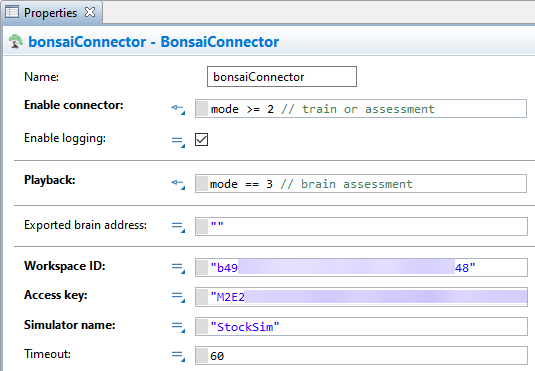
The completed Bonsai Connector
5. Creating and Training a New Brain
Before we can start training, we’ll need to first create the Inkling code that will be used as the brain’s training regimen. Instead of creating an empty brain and needing to manually define the RL object types, we’ll use a useful Bonsai feature that will generate a mostly complete Inkling code from a connected simulation model.
5a. Starting the Local Experiment
In this first part, we’ll connect our local model to the Bonsai platform.
-
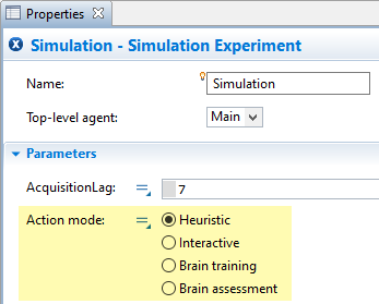
Configure the properties of the Simulation experiment, as follows (shown in the image below):
-
Ensure the option for “Skip experiment screen” is checked
-
The mode parameter is set to “Brain training” mode
-
Under the “Model time” section, set execution to “Virtual time” and the “Stop” condition to “Never”
-
Under the “Randomness” section, choose the option for “Random seed”
-
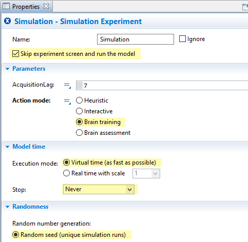
Relevant Simulation properties for starting locally hosted training
-
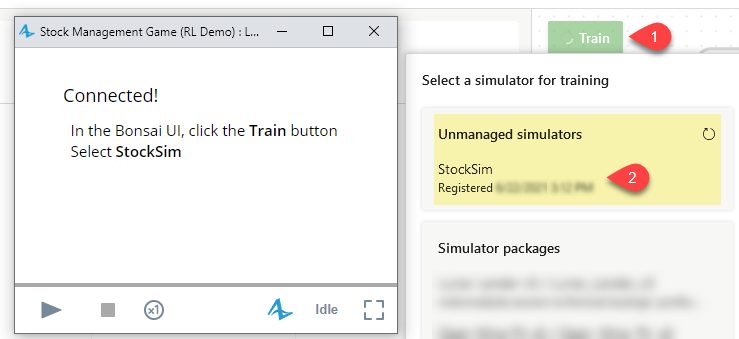
Launch the experiment; the Bonsai Connector should take over your model and display a “Connecting…”/“Connected!” message.
-
If “logging” is enabled in the Bonsai Connector, you can verify the connection is successful if the console contains a “Registered” line at the beginning and then reports a series of cyclical events reporting “Idle”-typed responses.
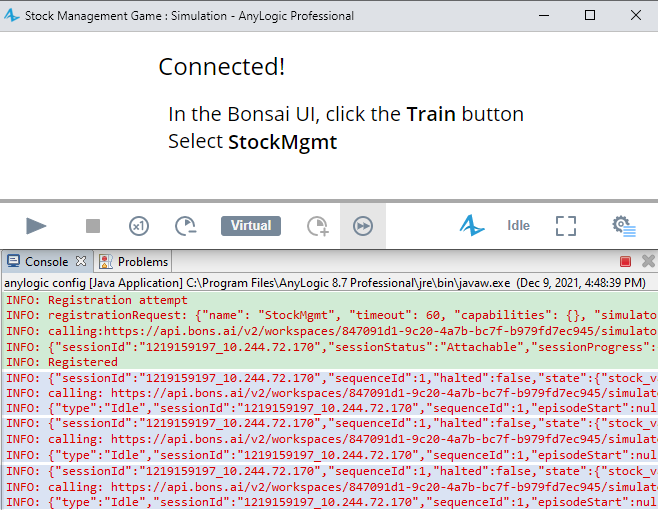
A successful connection (registration process is in green and idle
messages in blue)
Note: Timestamps for log statements were cropped out for brevity
5b. Creating a new Brain
-
Outside of AnyLogic, navigate to the Bonsai webapp within a web browser.
-
In the left panel, under “Simulators”, click on your named simulator with the “Unmanaged” label underneath it.
-
In the Info tab that appears, click on the “Create brain” button and give it a desired name.
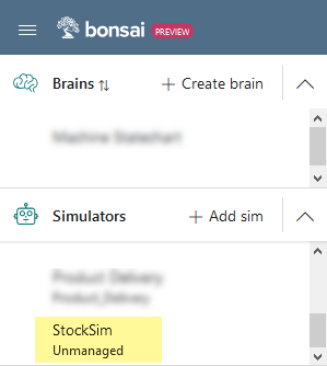
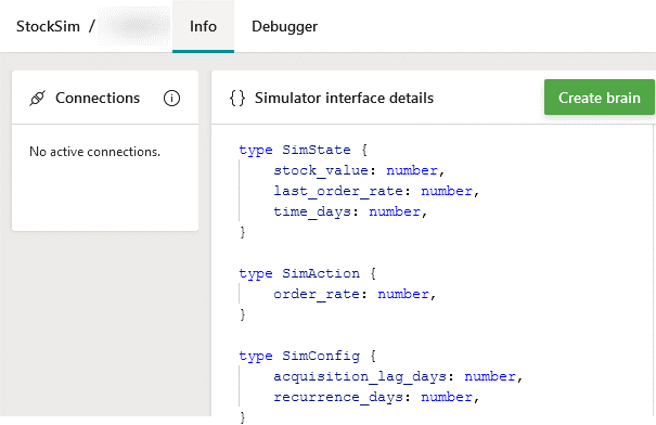
Locating and finding information on the sim from the Bonsai webapp
After the brain is created, you should see mostly complete Inkling code – primarily missing the feedback mechanism.
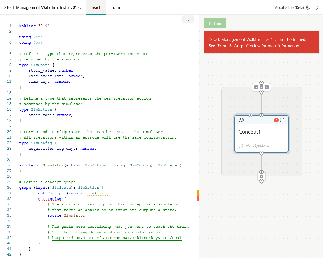
The Inkling code generated from the sim
5b-i. Setting up method of brain feedback
You have a choice for how to setup the feedback mechanism to the brain – reward/terminal functions or goals (they are mutually exclusive from one another).
This walkthrough will explain both, but later instructions will have screenshots/references to using goals. Instructions will remain the same, but the graphs and numbers in assessment results will differ.
After you try one method, create a new version of the brain (right click > “Copy this version”) or create a new brain, and then try with the other – experiment to see how results differ!
Method 1: Reward/Terminal functions
To devise the reward function, we have to consider how to convert the state of the simulation (at the time of an iteration) into a form of numerical feedback to give the brain an indication of the performance of its past action. The reward function is queried at the start of an iteration and formulated from the current observation.
In this example, the reward should be positive when it’s kept in the desired range (1000 – 3000) and negative when it’s outside. We’ll incentivize it to get it towards the middle by giving a larger positive reward in the middle; to simplify the math, this will decrease linearly.
In the implementation, we’ll normalize the numerical feedback by constraining the reward to [-1, +1] range. The best score (+1) is given when the stock level is in the middle of the allowed range (2000). A neutral score (0) is given when the stock level is at the extremes of the range (1000 or 3000). The reward will then continue below zero linearly, as the stock level gets lower than 1000 or higher than 3000, with the minimum -1. A graphical representation of this can be seen in the below image.
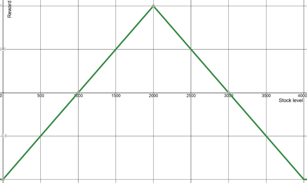
Graphical representation of the reward given on each iteration based on stock level
-
If not present, include the Math library (reference) by adding the line `using Math` to your Inkling code.
-
Define a new function (e.g., “GetReward”) that takes the simulator’s state as input and returns the following code:
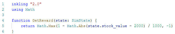
Implementation of the reward function
At the start of each iteration, the received observation is also passed to the terminal function to determine whether the current episode (or simulation run) should terminate, allowing the next to begin.
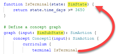
- Define a new function (e.g., “IsTerminal”) that takes the simulator’s state as input and returns a boolean expression evaluating as true when the value of time_days is greater than or equal to 3650 days (i.e., approximately 10 years).
This episode length was chosen based on it being a reasonable timeframe that also gives the brain a decent number of samples to learn from (3650 days / 50 days between episodes = 73 iterations).
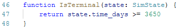
Implementation of the terminal function
- Inside the concept graph, under the curriculum statement, reference the names of the reward and terminal functions via the reward and terminal keywords.
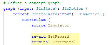
Reference to the reward/terminal functions
Method 2: Goal statements
To setup goals, we just need to use the proper syntax to describe what we want the brain to achieve using Bonsai’s available objective types.
In this case, we want the brain to get the stock value into the desired range [1000 – 3000] and then keep it there for the duration of the episode; this aligns with the “drive”-typed goal (reference).
-
Ensure you have the goal library imported by including the line `using Goal` in your Inkling code.
-
In the concept graph, under the curriculum clause, include the `goal` statement and define a `drive` goal (e.g., “JustRight”) with the condition that the stock value is between 1000 and 3000.
- (OPTIONAL) Include a `within` statement at the end, limiting it to a reasonable number of iterations (e.g., 3)
The name “JustRight” stems from the idea that the range [1000 – 3000] is desirable and leaves the stock at a level that’s not too low or excessively high.
The specific value of 3 for the optional “within” statement was chosen arbitrarily.
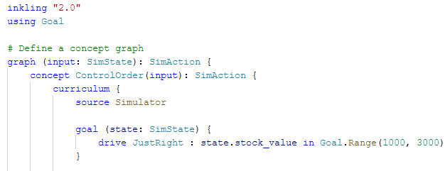
The goal definition without the `within` statement
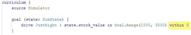
The goal definition with the `within` statement
If you do not include the `within` statement, each episode will run for 1000 iterations; in this model, that equates to 1000 * 50 days = 50,000 days or about 137 years! Having it run for this long is not necessarily negative, as the concept of time is somewhat irrelevant in this toy model. Since the important aspect to enforce is simply teaching the brain how to stay inside the range, it may be a needless constraint to limit the episode time any further. However, one scenario we do want to avoid is if, as part of the training, the brain gets out of control and ends up spending dozens of simulated years going far outside the range.
5b-ii. Declaring a Lesson (Configuration)
In general, lessons in Inkling allow you to “provide a staged way to teach a concept” (reference: Bonsai documentation). Of relevance to this example is that they are where you specify values for the Configuration. These are passed to the model at the start of each training episode.
Critical: If you omit adding a lesson (and thus specifying Configuration values), the model will use the Java default values (0 for numerical types, null for arrays or objects). This may cause unexpected behavior or possibly errors in your model, assuming this case is not handled in your Configuration code area.
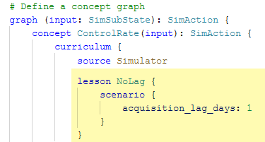
In this example, we will add the lesson called “NoLag”, declaring a scenario where our previously defined configuration value (`acquisition_lag_days`) is set to 1. This is added as part of the curriculum.
The name “NoLag” is used to indicate that the amount chosen by the brain will be received by the model immediately.
5b-iii. Defining Constraints
In Inkling, you can define numerical ranges or enumerated sets that values in your type objects should be constrained to (reference: Bonsai Documentation).
Your action type should have constraints to inform the brain what are the valid ranges it can take – otherwise it will use the full range of floating point 32-bit numbers!
Optionally, the observation/state can have constraints; including them may have some training benefits (e.g., faster training or more likely to converge on a successful policy).
Critical: If your model sends values outside the ranges/options defined, Bonsai will throw warnings during training; exported brains also adhere to these constraints and will throw errors if you try to pass any other values. It’s advised to only set constraints that will not change over time.
Optionally, the configuration type can also have constraints; including them will serve as validation in your scenario descriptions in subsequent steps, but otherwise have no effect on training or the model.
In this model, we can define the following constraints (see the images below for the code):
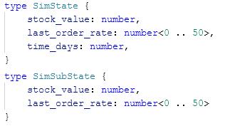
- For `order_rate` in the SimAction - also `last_order_rate` in SimState - the range is continuous and between 0 and 50.
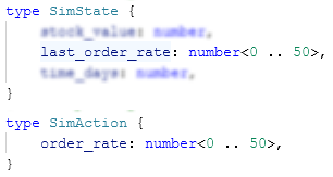
Constraint for state and action
Depending on how you setup the training regimen (e.g., maximum iterations per episode, choice of reward/terminal or goals), the ranges for stock value and time can vary greatly. To minimize the potential for warnings/errors later on, they’re left unconstrained; this should have a negligible effect on training.
- (OPTIONAL) Add a constraint to the Configuration’s acquisition_lag_days with the range 1 to 7, with a step size of 1.
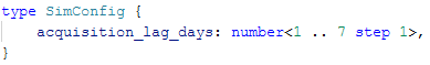
Constraint for Configuration
Adding configuration constraints prevents a brain to be trained if a lesson attempts to define values outside this range. The lower bound (1) is especially important in this case, as having values less than 1 will cause logical errors in the model (as the value is used as part of a mathematical operation).
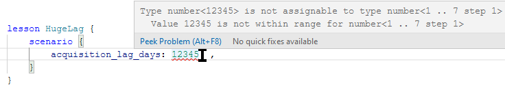
Example result of invalidating Configuration constraints
5b-iv. Applying State Transformation
Another useful Bonsai feature allows us to use a subset of state values for the brain; essentially this works like a filter (further reference: Bonsai documentation).
In other words, we can setup the Observation section of the RL Experiment with as many relevant data points that we might wish to use in any part of the Inkling code (e.g., reward, terminal, goal, state). We can then choose (and experiment with) sending a subset of these data points to the brain for what it should be trained with.
For this model, we included the current model time so that we could use it in the logic of the terminal function. In addition to being irrelevant for the brain’s decision to choose an action, it would also not apply if we eventually wanted to deploy this in a real system (as the idea of simulated time doesn’t carry over to the real world) – thus, it’s ideal to filter this out.
-
Duplicate the “SimState” type definition (e.g., copy/paste it below the original) and change the name accordingly (e.g., “SimSubState”).
-
In the “sub-state” type, remove the value for time.
-
In the concept graph, change the type of input to reference the new type.
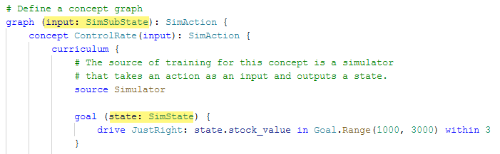
Any reward/terminal functions or goal statements can still use the original, full state (and thus any values within the type).
For an example, see the image below. Note the different type references between the graph’s input and the terminal function’s input; the graph input is what the brain receives, whereas the terminal function can receive the full set of values.
After doing this, you will also see the changes in the visual graph (as noted by the icon representing the state transform and the reduced number of inputs).
5c. Establishing the local connection
When your Inkling code is setup, the connection is ready to be made.
-
Ensure your model is running and still showing the “Connected!” message (if not, repeat the steps to start the local training experiment)
-
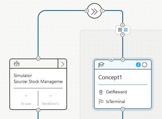
In the Bonsai UI, with your brain’s desired version selected, click the green “Train” button. In the pop-up, select your simulator from the list of “Unmanaged simulators”. The pop-up will dismiss, and - after a few seconds - it should connect to your simulation model and begin training!
During this time, you will see your model automatically starting, running itself, and restarting. For new versions of a brain, it will run your simulation model for a few iterations before taking a minute or so to fully initialize the brain. Expect some short delays at the start and after every few dozen or hundred episodes as the brain updates its internal policy and runs automatic assessments.
Critical: During training, it is important not to make any meaningful action in the animated model. For example, attempting to pause the simulation manually may cause the Bonsai Connector to misinterpret the action as a prompt to take an action. During locally hosted training, it’s most important to watch for any errors from the simulation model or from the Bonsai UI.
6. Uploading the model for rapid training sessions
Once you’re confident that there are no errors present, you may wish to export the model and upload it to Azure.
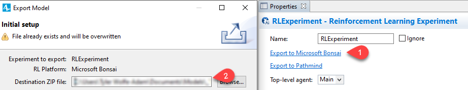
- Inside of AnyLogic, click the “Export to Microsoft Bonsai” inside the properties of your RL experiment and choose a desired save location.
-
Inside of the Bonsai platform, in the “Simulators” panel on the left, click “+Add Sim”, then on AnyLogic.
-
Select or drag and drop your exported model and give the Simulator a name, then click “Create simulator”.
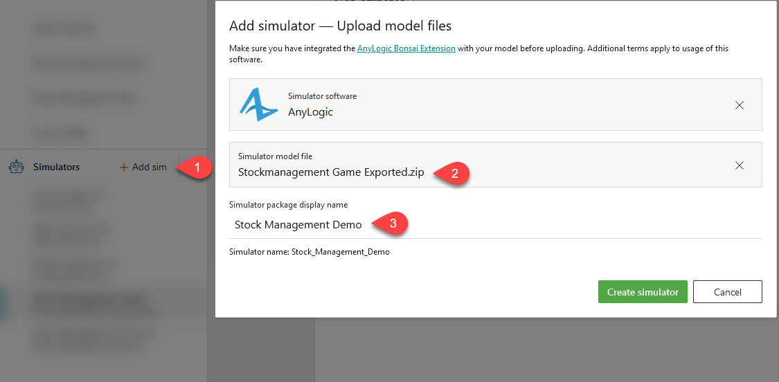
Your model will get uploaded, then wrapped in a Docker container. After it’s finished, you’ll get a chance to configure the environment settings (e.g., max instance count, cores, memory) – if you change these settings, remember to hit the “Apply” button.
Because you already have a brain setup, you do not need to create a new brain. Instead, we’ll reference this uploaded model from your current brain.
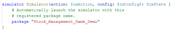
- In the “Info” tab of your uploaded model, click on the “Copy” button next to the package name (circled in purple in the image below).
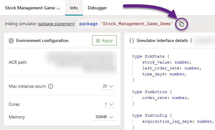
- Go to your Inkling, find the “simulator” clause and paste your package reference inside of it. This will cause Bonsai to always use that simulator whenever you start the training.
- Click on the green “Train” button. Bonsai will then start to spin up multiple instances of your model – the maximum of which is based on the environment settings.
During training, you can see a live update of the observations and actions being taken from the “Train” tab. More information can be read about from Bonsai’s documentation: https://docs.microsoft.com/en-us/bonsai/tutorials/evaluate-assessment.
7. Performing Assessments on the Brain
To evaluate the performance of the trained brain, there are a few options.
Bonsai has a built-in “Custom Assessment” feature that lets you test how well the brain performs in relation to the goal/reward mechanism you setup for training. This is accomplished entirely on the Bonsai webapp. More information can be read from the Bonsai documentation: https://docs.microsoft.com/en-us/bonsai/guides/assess-brain
You may also decide to export the brain, then hosting it locally (via Docker) or on an Azure webapp. You can then paste the prediction endpoint in your Bonsai Connector object and run your Simulation experiment with the “Assessment”/”Playback” mode selected. For more information on the export options, see the Bonsai documentation: https://docs.microsoft.com/en-us/bonsai/guides/export-brain?tabs=docker-ps&pivots=brain-api-1
8. Final remarks / Iterating on the model
Given that this is a toy model, there is a lot of room for improvements in features and functionality – both on the simulation side and the Inkling side.
In the model, there is an event that controls the exogenous demand, called “ExogenousDemandChange”, updating it by ± 1 every day. While it has a limit on how low the demand can be (0), it has none for the upper limit, meaning it can eventually grow up to infinity (the likelihood of which increases the longer the episode runs for). If it gets past 50 – the highest the brain can set an order rate – the brain will ultimately be unable to keep up, causing it to get penalized for a scenario that’s impossible to overcome!
One resolution on the simulation-side is to modify the logic of the event. We can use AnyLogic’s built-in limit function to constrain the rate’s lower and upper bound. This can be done by changing the code to read: Demand = limit(0, Demand + uniform( -1, 1 ), 50);
Another resolution can be done on the Inkling side, particularly when using goals. Since we know each action is 50 days apart, we can limit the max iteration to end the simulation run after a reasonable amount of time – say, to 146 (~20 years). This can be done by adding a training clause to the curriculum clause and setting the EpisodeIterationLimit parameter (reference: Bonsai documentation).
Additionally, there are a multitude of other Inkling related variants that may improve the results. These might include:
-
Only passing the stock value to the brain (not the last order rate)
-
Allowing a higher (or even lower) “within” tolerance to the “drive” goal
-
Splitting the one goal into multiple (e.g., adding an avoid-type goal to include another terminating condition)
-
Using a non-linear reward function
Appendix: Full Inkling Code
The following is the completed Inkling code.
It uses goals as the form of brain feedback, but the reward and terminal functions are also included as well. To have the brain train with these instead, you can - inside of the Bonsai webapp - simply comment out the lines involved in the “goal” statement and uncomment the lines for the “reward” and “terminal” statements (both of which are in the concept graph).
inkling "2.0"

using Math

using Goal

\# Define a type that represents the per-iteration state

\#   returned by the simulator.

type SimState {

    stock_value: number,

    last_order_rate: number\<0 .. 50\>,

    time_days: number,

}

\# Define the "sub-state" or the state which will be

\#   observed by the brain.

type SimSubState {

    stock_value: number,

    last_order_rate: number\<0 .. 50\>

}

\# Define a type that represents the per-iteration action

\#   accepted by the simulator.

type SimAction {

    order_rate: number\<0 .. 50\>,

}

\# Per-episode configuration that can be sent to the simulator.

\# All iterations within an episode will use the same configuration.

type SimConfig {

    acquisition_lag_days: number\<1 .. 7 step 1\>,

}

\# Define the input/output types to the simulator,

\# and optionally the simulator package (for managed/scaled sims).

simulator Simulator(action: SimAction, config: SimConfig): SimState {

    #package "Stock_Management_Demo"

}

\# Define the numerical feedback for the brain,

\#   which judges the performance of the last action based on the current state.

\# (This won't be called if you're using goals)

function GetReward(state: SimState): number {

    return Math.Max(1 -  (Math.Abs(state.stock_value-2000)) / 1000,-1)

}

\# Define a condition for when an episode should be terminated,

\#   allowing the next to begin.

\# (This won't be called if you're using goals)

function IsTerminal(state: SimState) {

    return state.time_days \>= 7300

}

\# Define a concept graph.

\# With the values that the brain receives based on the ‘input’ type.

graph (input: SimSubState): SimAction {

    concept Concept1(input): SimAction {

        curriculum {

            # The source of training for this concept is a simulator

            # that takes an action as an input and outputs a state.

            source Simulator

            # Initial lesson to teach the brain.

            # It describes a scenario, defining the Configuration values to use.

            lesson NoLag {

                scenario {

                    acquisition_lag_days: 1

                }

            }

            # Reference the defined reward/terminal functions.

            # Only uncomment the following two lines if not using goals.

            #reward GetReward

            #terminal IsTerminal

            # Add goals here describing what you want to teach the brain

            # See the Inkling documentation for goals syntax

            # https://docs.microsoft.com/bonsai/inkling/keywords/goal

            goal (state: SimState) {

                drive JustRight: state.stock_value in Goal.Range(1000,
3000) within 3

            }

        }

    }

}