How to identify potential predictors for survey results using information value
Simone Liebal
2020-11-25
Source:vignettes/IV-report.Rmd
IV-report.RmdAbout
This post will give you a short introduction to the data exploration technique information Value (IV) and how to use it as part of the wpa R package.
After setting the stage, we will have a look at how this can be used to identify potential predictors for survey responses.
What is Information Value?
Information Value (IV) refers to a data exploration technique that helps determine which variables in a dataset have predictive power or influence on the value of a dependent variable. This technique delivers an IV score, which in itself tells you whether one variable A is a good predictor for another (say B). If A has a low information value, it is potentially not be a good predictor for variable B, and vice versa. Unlike other methods of measuring relationship between variables, such as correlation or simple linear regression, the IV score is calculated with in terms of how well a specific variable A can distinguish between a binary response in a target variable B.
Or said differently:
Imagine you have you have a simple yes/no question, e.g. “Are you satisfied with your current work-life-balance?”. The answer to that question, which only has two possible values, is defined as variable B, and each value in that variable as b. We also have a variable A, which is the average weekly total of after-hours collaboration time, and each value in A is denoted as a.
Let’s assume the values for a and b are captured for 10000 employees, and are contained in the two variable-columns A and B. On a row-wise basis, each a in A links to a b in B. Based on these values, the information value for A can be calculated.
For this purpose, data is separated into different buckets or bins, with the same quantity of data (responses) in each of them. Here we are choosing 5 bins, therefore 20% of responses in each of them.
The numbers and distributions in this example are exaggerated for illustrative purposes:
| Avg. weekly after-hours | Total # of responses | # of negative responses | # of positive responses |
|---|---|---|---|
| 0-2 | 2000 | 200 | 1800 |
| 2-4 | 2000 | 350 | 1650 |
| 4-6 | 2000 | 800 | 1200 |
| 6-8 | 2000 | 1200 | 800 |
| 8-10 | 2000 | 1400 | 600 |
The information value is then calculated using the following formula:
A component in calculating IV is the Weight of Evidence (WoE), which is the logarithmic part within the formula above:
WOE describes the relationship between a predictor variable and a binary target variable for each bin, while IV measures the strength of that total relationship across all the bins.
Applying this to the table above, we get the following:
| Avg. weekly after-hours | Total # of responses | # of negative responses | # of positive responses | WOE |
|---|---|---|---|---|
| 0-2 | 2000 | 200 | 1800 | 1.438 |
| 2-4 | 2000 | 350 | 1650 | 0.791 |
| 4-6 | 2000 | 800 | 1200 | -0.354 |
| 6-8 | 2000 | 1200 | 800 | -1.165 |
| 8-10 | 2000 | 1400 | 600 | -1.607 |
The first two bins (0-2 and 2-4) show a
positive WOE value. This means the percentage of positive
responses is higher than the percentage of negative
responses. For the other three bins (4-6,
6-8, and 8-10), we can observe a negative WOE
value, which means that the percentage of “negative responses” is higher
than the percentage of “positive responses”. Therefore, respondents with
0 to 4h in average weekly after-hours seem to answer more positively on
the work-life-balance question.
With the WOE calculated, we can apply the full IV calculation to the table:
| Avg. weekly after-hours | Total # of responses | # of negative responses | # of positive responses | WOE | IV |
|---|---|---|---|---|---|
| 0-2 | 2000 | 200 | 1800 | 1.438 | 0.3621 |
| 2-4 | 2000 | 350 | 1650 | 0.791 | 0.1309 |
| 4-6 | 2000 | 800 | 1200 | -0.354 | 0.0331 |
| 6-8 | 2000 | 1200 | 800 | -1.165 | 0.3772 |
| 8-10 | 2000 | 1400 | 600 | -1.607 | 0.7053 |
In terms of predictiveness you can use the following table as a reference:
| IV value | predictiveness |
|---|---|
| Less than 0.02 | Not useful for prediction |
| 0.02 to 0.1 | Weak predictive power |
| 0.1 to 0.3 | Medium predictive power |
| 0.3 to 1.0 | Strong predictive power |
| > 1.0 | Very strong predictive power |
Therefore in this example, after-hours seem to have a strong predictive power regarding the answer to “Are you satisfied with your current work-life-balance?”. This data exploration technique builds the foundation for predictor analysis using the wpa R package.
Let’s get started
As of writing this article, there are two IV functions included as
part of the wpa R package - create_IV()
and IV_report(). To run either of those, you will need to
ensure that the package has been successfully installed for your version
of R. For more information on the installation process, please check out
https://microsoft.github.io/wpa.
Putting it into practice
create_IV() function
Let’s start with create_IV(). For data input, the
create_IV() function uses a standard person query dataset.
The wpa package already brings a set of built-in
datasets for testing purposes. The ready-to-use standard person query
dataset is called sq_data and will be used for this section
of the post.
To get started, open a new session in R and load the following packages:
The general format looks like this:
create_IV(
    data,
    predictors = NULL,
    outcome,
    bins = 5,
    return = "plot")
At minimum, you need to supply the data argument, which
is a Person Query dataset in the form of a data frame and the variable
you want to calculate the IV for (outcome) to run the
report. If only these two are defined, the remaining arguments will use
default values.
Additionally, it’s recommended to use the predictors
argument to specify specific columns, that you want to include.
Otherwise, all numeric vectors in the data will be included, which might
lead to a rather big output.
You can also adjust what the output will look like with the
return argument - here you have a choice of:
- “plot” (returns a bar plot)
- “summary” (returns a summary table)
- “list” (returns a list of outputs for all input variables)
- “plot-WOE” (returns a WOE plot)
bins allows you to define the amount of same-sized bins
the data is separated into.
Using the sq_data dataset, you can have a look at the
predictors focus hours, email hours and meeting hours in correlation to
collaboration hours:
sq_data %>%
    mutate(X = ifelse(Collaboration_hours > 12, 1, 0)) %>%
    create_IV(
        outcome = "X",
        predictors = c("Email_hours", "Meeting_hours", "Total_focus_hours"),
        return = "plot")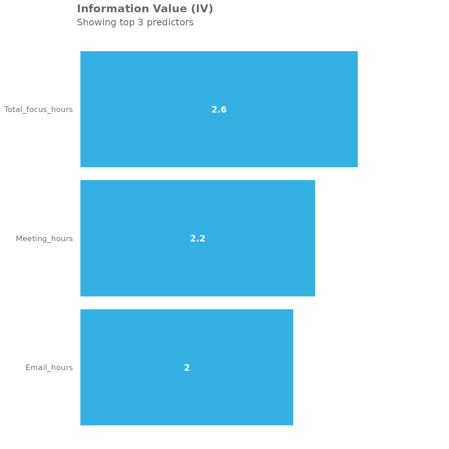
You may see, that all three are very strong predictors. Initially it
might come as a bit of a surprise, that Total_focus_hours
is actually the strongest predictor of those three, even though focus
hours (in the context of Workplace Analytics) are a block of at least
two hours without any meetings - so pretty much the opposite of
Collaboration_hours.
This is where WOE comes into play, as it describes the relationship between a predictor variable and a binary target variable:
sq_data %>%
    mutate(X = ifelse(Collaboration_hours > 12, 1, 0)) %>%
    create_IV(outcome = "X",
    predictors = c("Email_hours", "Meeting_hours", "Total_focus_hours"),
    return = "plot-WOE")
#> [[1]]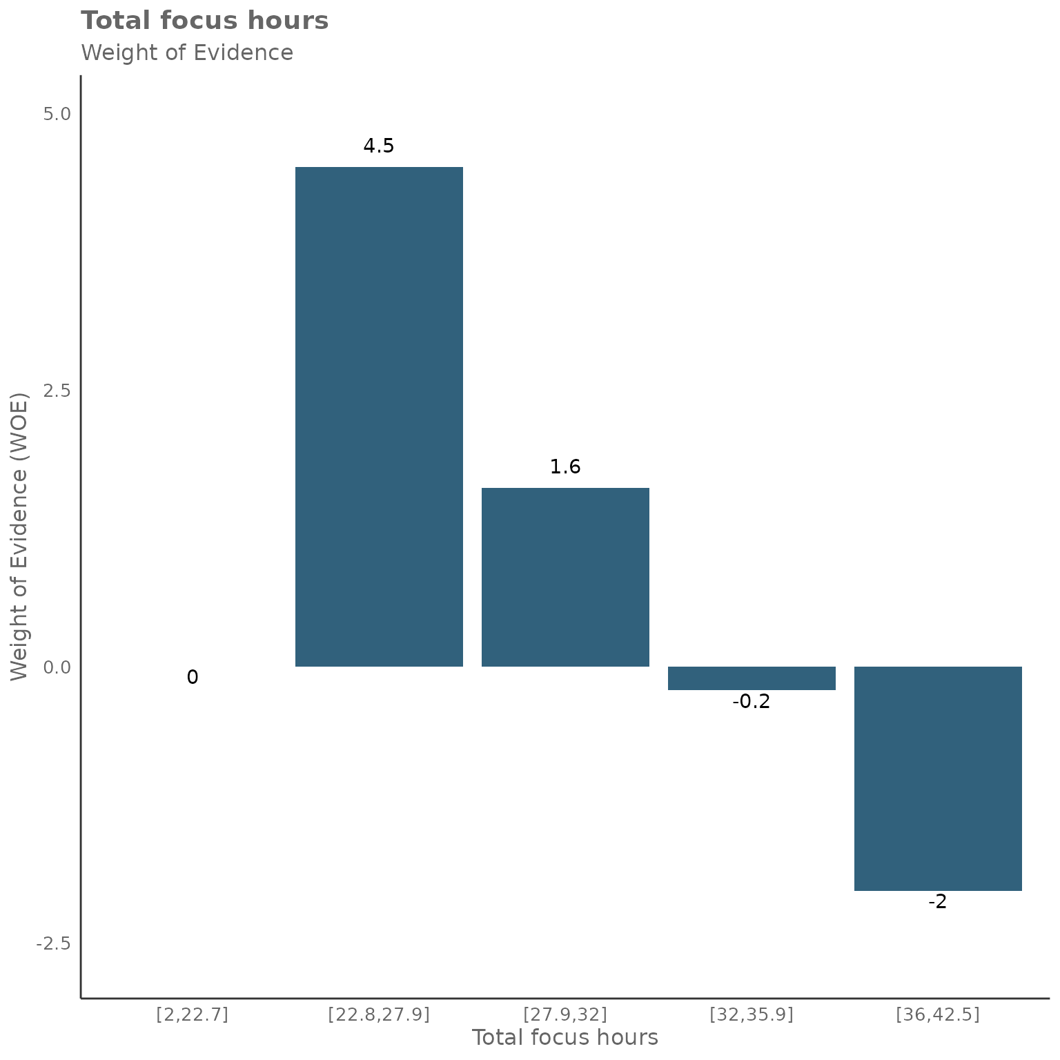
#>
#> [[2]]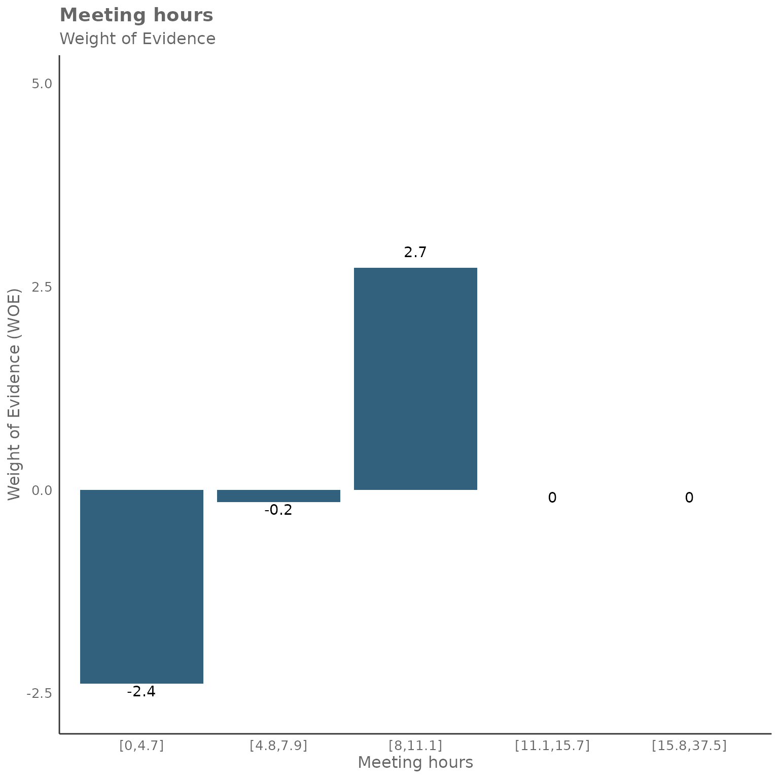
#>
#> [[3]]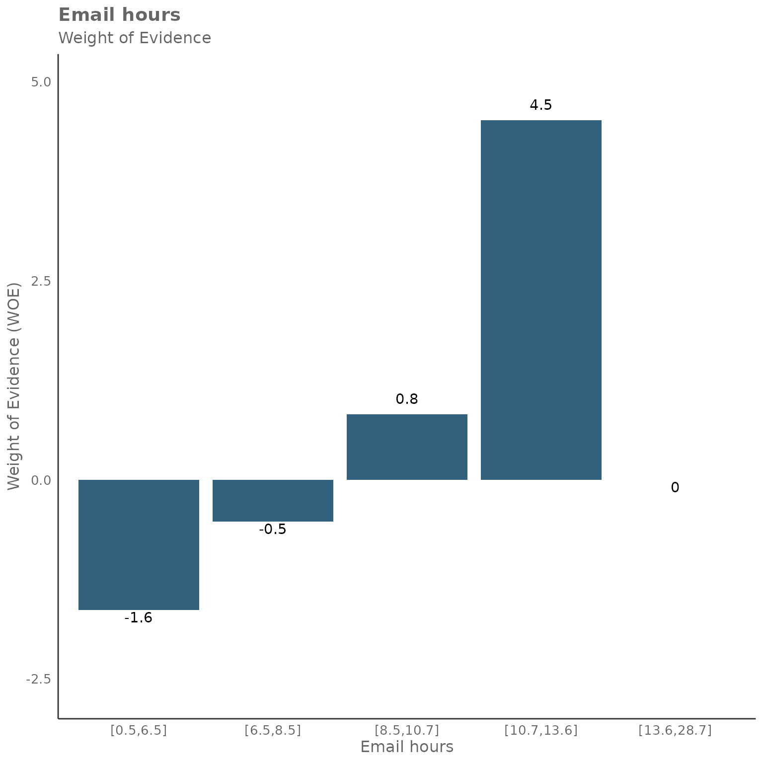
You may see, that meeting hours and email hours seem to have direct relationship with collaboration hours:
Focusing on email hours as an example - we have the buckets with the lower email hours to the left and the higher ones to the right.
The two buckets on the left have a negative WOE value. This tells us, that less email hours seem to lead to less collaboration hours.
The two buckets on the right have a positive WOE value. This tells us, that more email hours seem to lead to more collaboration hours.
But what about the focus hours?
Focusing on the WOE chart for focus hours above, we can see an inverse relationship. Again, we have low amount of focus hours on the left and high amount of focus hours on the right.
The two buckets on the left have a strong positive WOE value. So, less focus hours seems to have a correlation with more collaboration hours and vice versa.
Working with categorical predictors
The create_IV() function is not limited to numeric
predictors - it can also handle categorical variables such as
organizational attributes or job functions. This is particularly
valuable when exploring how different groups within an organization
might relate to specific outcomes.
Let’s explore how categorical predictors like
FunctionType and LevelDesignation might
predict high collaboration patterns:
sq_data %>%
    mutate(High_collab = ifelse(Collaboration_hours > 12, 1, 0)) %>%
    create_IV(
        outcome = "High_collab",
        predictors = c("FunctionType", "LevelDesignation", "Organization"),
        return = "plot")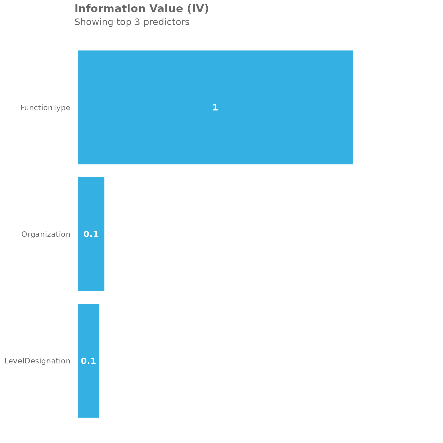
The plot shows the Information Value scores for these categorical predictors. You can see that different organizational attributes have varying predictive power for high collaboration patterns.
To get more detailed insights, let’s examine the summary table:
sq_data %>%
    mutate(High_collab = ifelse(Collaboration_hours > 12, 1, 0)) %>%
    create_IV(
        outcome = "High_collab",
        predictors = c("FunctionType", "LevelDesignation", "Organization"),
        return = "summary")
#>           Variable         IV
#> 1     FunctionType 0.96044276
#> 2     Organization 0.09296163
#> 3 LevelDesignation 0.07416827
The summary table provides the exact IV values, allowing you to quantify the predictive strength of each categorical variable. Based on our earlier reference table:
- IV < 0.02: Not useful for prediction
-
IV 0.02-0.1: Weak predictive power
- IV 0.1-0.3: Medium predictive power
- IV 0.3-1.0: Strong predictive power
You can also examine the Weight of Evidence (WOE) patterns for categorical predictors to understand how different categories within each variable relate to the outcome:
sq_data %>%
    mutate(High_collab = ifelse(Collaboration_hours > 12, 1, 0)) %>%
    create_IV(
        outcome = "High_collab",
        predictors = c("FunctionType", "LevelDesignation"),
        return = "plot-WOE")
#> [[1]]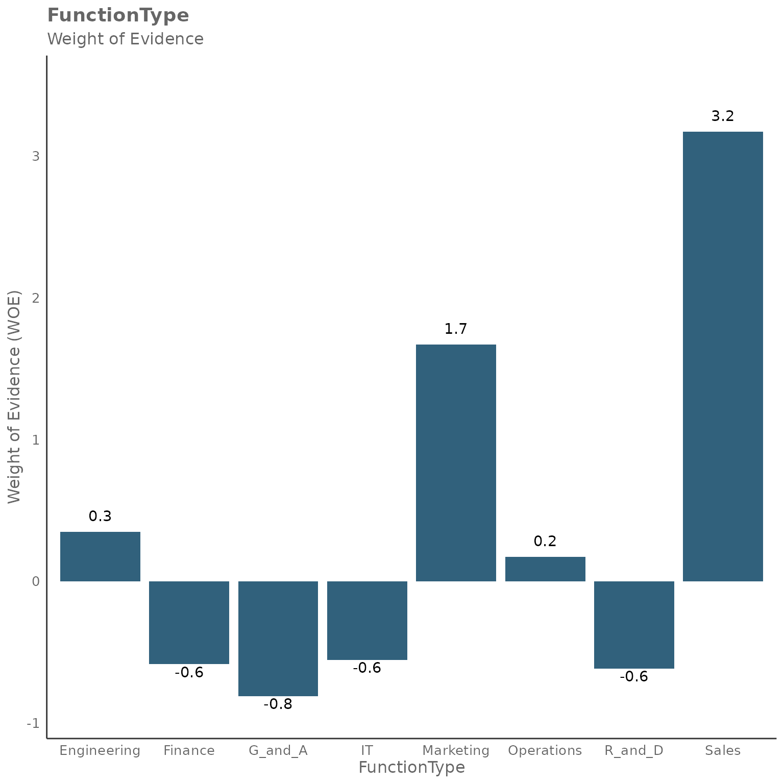
#>
#> [[2]]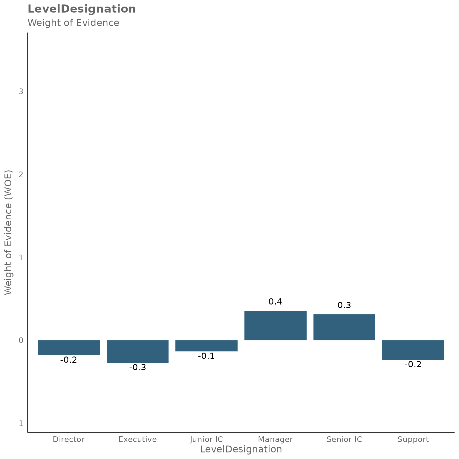
The WOE plots for categorical variables show how each category (e.g., different function types or organizational levels) contributes to predicting the outcome. Positive WOE values indicate that category is more associated with high collaboration (outcome = 1), while negative WOE values suggest lower collaboration patterns.
Combining numeric and categorical predictors
One of the strengths of the IV approach is that you can easily combine both numeric and categorical predictors in a single analysis:
sq_data %>%
    mutate(High_collab = ifelse(Collaboration_hours > 12, 1, 0)) %>%
    create_IV(
        outcome = "High_collab",
        predictors = c("Email_hours", "Meeting_hours", "FunctionType", "LevelDesignation"),
        return = "plot")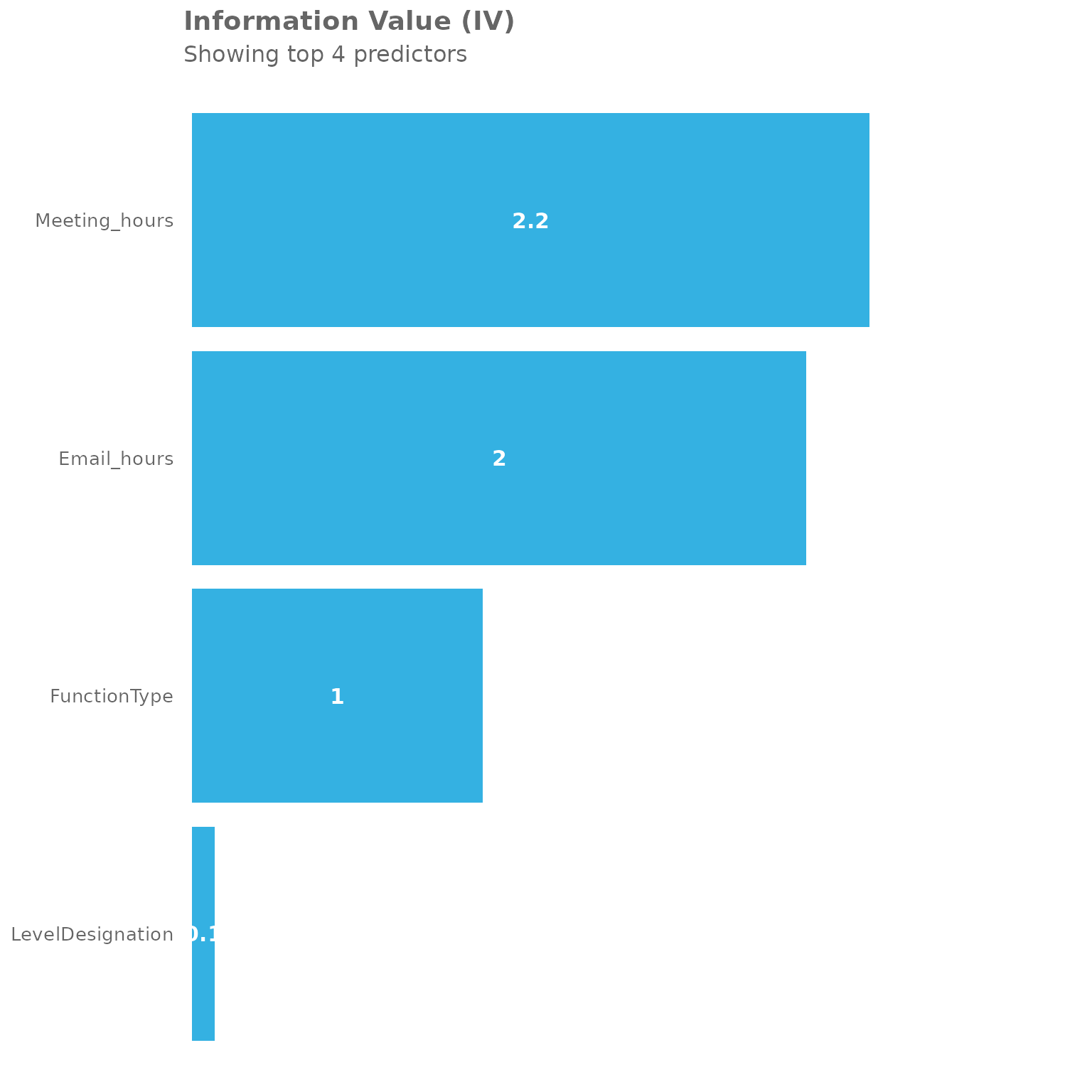
This mixed approach gives you a comprehensive view of which factors - whether behavioral (like email/meeting hours) or organizational (like function type) - are most predictive of your outcome of interest.
IV_report() function
Another option is the IV_report() function, which
generates an interactive HTML report, again using Standard Query data as
an input. The report contains a full Information Value analysis.
This function follows a similar format as the
create_IV() function above, with the difference that the
return is already predefined as an HTML report. Instead it
consists of two other additional arguments - path, which
defines the file path and the desired file name and
timestamp, which is a true/false variable that defines
whether to include a time stamp in the file name.
The general format is the following:
IV_report(
    data,
    predictors = NULL,
    outcome,
    bins = 5,
    path = "IV_report",
    timestamp = TRUE)
Using the IV report with survey results
The IV report can be leveraged as a powerful option to identify potential predictors for survey responses. In this section we will focus on the non-free-text responses. Our example will use survey responses on a scale from 1-5 (1 being most disagreeable - 5 being most agreeable).
To get started, the survey responses need to uploaded as an additional column (per question) to the organizational file, that is uploaded via the Workplace Analytics portal. You can find more information on the upload of that data here.
After creating a new standard person query, which includes the new
column, the data can be imported using the import_wpa()
function into a new R session with the above mentioned libraries already
imported.
raw_data <- import_wpa(myfile)The query data might include multiple lines per person per time period. In this example, we only have the current survey responses available. To simplify the analysis, these lines can be grouped by person ID with the result of only having one line per person going forward.
survey_data <- raw_data %>%
      group_by(PersonId) %>%
      summarise_if(is.numeric, mean, na.rm = TRUE)
Dealing with non-numeric values
The values used for the creation of IV and IV report need to be numeric. However when uploading the survey responses using the org-data file, these responses might be formatted as a string, even if they seem to be numeric at first glance.
Therefore, they need to be converted:
Convert answers into binary
The create_IV() and IV_report() functions
require the value of the outcome argument to be binary. A way to
approach this can be to convert all agreeable answers into “1” and all
disagreeable answers into “0”. In this example, we are working with a
scale from 1-5, which allows for a neutral answer with “3”. As this
response has limited value for predicting agreeableness or
disagreeableness, you can filter this out.
Create an outcome variable by turning survey answers into 1s and 0s (and neutral into 2):
survey_data$my_outcome <-
    ifelse(survey_data$survey_response_1 == "5", 1,
    ifelse(survey_data$survey_response_1 == "4", 1,
    ifelse(survey_data$survey_response_1 == "3", 2,
    ifelse(survey_data$survey_response_1 == "2", 0,
    ifelse(survey_data$survey_response_1 == "1", 0, 2) ) )))
Then, you can easily filter out the neutral answers:
Create IV and IV Report
With all the groundwork being done, you can now create the IV and IV report for this specific question (survey_response_1) to see what WPA metrics might be a predictor for the responses.
To create the IV:
To run the IV report:
IV_data %>% IV_report(
    outcome = "my_outcome",
    path="survey_response_1",
    predictors=c("Collaboration_hours", "Call_hours", "Meeting_hours", "Instant_Message_hours", "Email_hours", "Workweek_span", "After_hours_instant_messages" ,  "After_hours_in_unscheduled_calls", "After_hours_collaboration_hours"))
This creates an IV report for the survey_response_1 of the whole
population. To dive deeper and identify trends for a specific a
population you can apply filters (e.g. LevelDesignation,
Organization, etc.) before creating the report.
For example, filtering by LevelDesignation:
Feedback
Hope you found this useful! If you have any suggestions or feedback, please visit https://github.com/microsoft/wpa/issues.