Getting started
This section contains the detailed installation instructions, and a first overview on how functions work in the wpa package.
Installation
The stable version of wpa can be installed directly from CRAN:
install.packages("wpa")There may occasionally be some experimental features that are only available in the development version. To install the development version from GitHub, you can also run:
# Check if remotes is installed, if not then install it
if(!"remotes" %in% installed.packages()){
  install.packages("remotes")
}
remotes::install_github(repo = "microsoft/wpa", upgrade = "never")
The above code will tell R not to update dependency packages, which speeds up the installation process. If you’d like to update all dependency packages, you can remove upgrade = "never" from the code. When prompted to update your packages, we recommend updating all CRAN packages.
As best practice, you should restart your R Session both before and after running the above code.
If you prefer to proceed with a local installation, you can download a installation file here.
Troubleshooting installation
If you encounter any issues with package installations, you can find the recommended troubleshooting flow below. Note that this process can take 10-15 minutes for a full package library update.
- Restart your R Session. Clear any objects in your workspace.
- Run
update.packages(ask = FALSE), which will update all the packages installed on your machine to the latest versions. If prompted to install from source any packages which require compilation, clickNo. All your installed packages should start updating, and this can take a while if you have many installed packages or if you have not updated them for a while. - Try installing the R package again with the command
devtools::install_git(url = "https://github.com/microsoft/wpa.git"). - Restart your R Session again and run your code.
Loading the wpa package
Once the installation is complete, you can load the package with:
You only need to install the package once; however, you will need to load it every time you start a new R session.
wpa is designed to work side by side with other Data Science R packages from tidyverse. We generally recommend to load that package too:
Importing Workplace Analytics data
To read data into R, you can use the import_wpa() function. This function accepts any query file in CSV format and performs variable type conversions optimized for Workplace Analytics.
Assuming you have a file called myquery.csv on your desktop, you can import it into R using:
setwd("C:/Users/myuser/Desktop/")
person_data <- import_wpa("myquery.csv")
In the code above, set_wd() will set the working directory to the Desktop, then import_wpa() will read the source CSV. Note that file paths in R must be provided as a forward-slash (/) or escaped back-slash (\\).
As an alternative to set_wd(), you may also consider using RStudio Projects, which enables you to use relative links within the working directory instead of set_wd() and full file paths.
The contents will be saved to the object person_data (using <- as an Assignment Operator).
Demo data
The wpa package includes a set of demo Workplace Analytics datasets that you can use to explore the functionality of this package. We will also use them extensively in this guide. The included datasets are:
-
sq_data: A Standard Person Query -
dv_data: A Standard Person Query with outliers -
mt_data: A Standard Meeting Query -
em_data: An Hourly Collaboration Query -
g2g_data: A Group-to-Group Query
See here for a full documentation of the queries in Workplace Analytics.
Exploring a person query
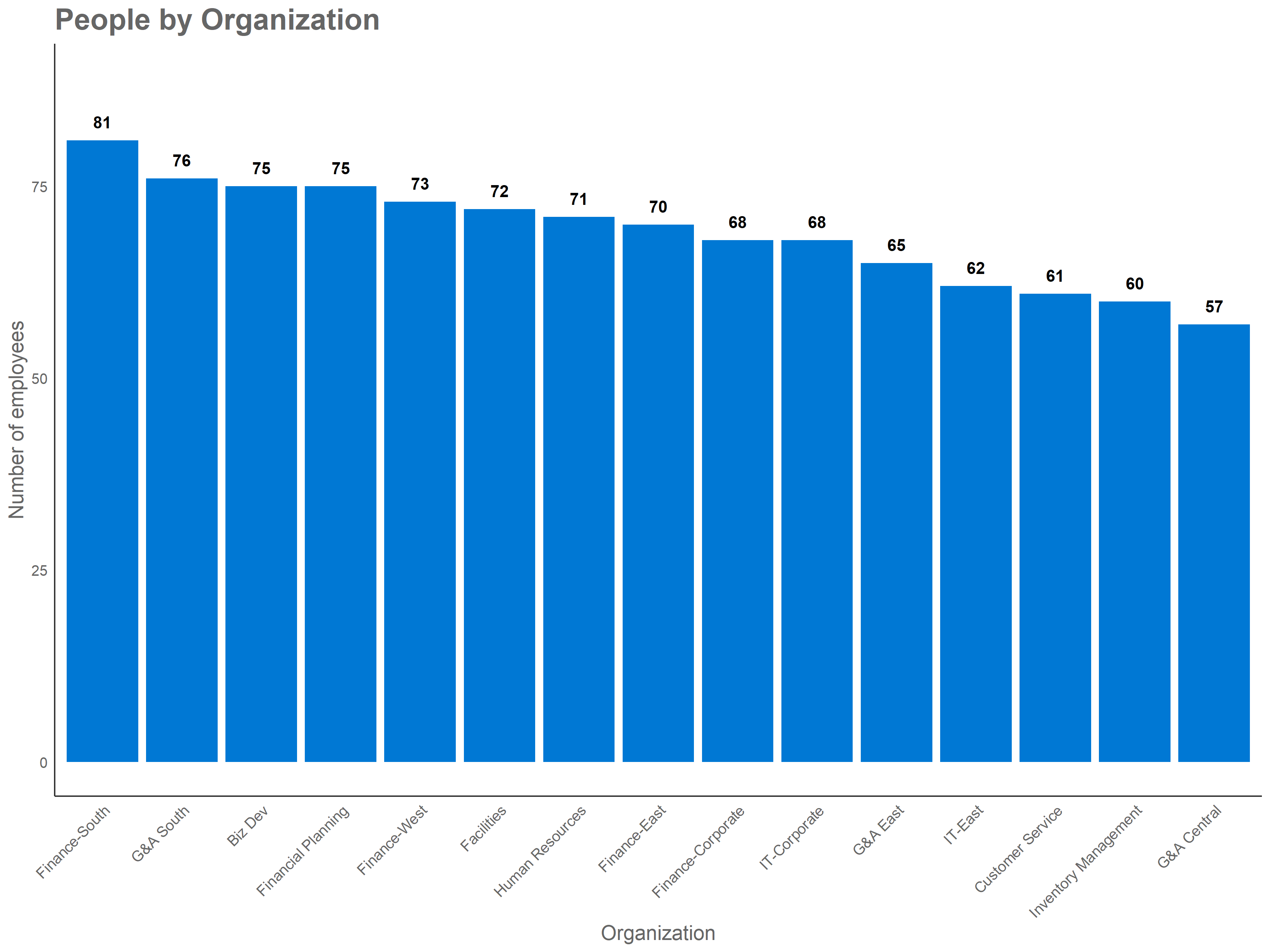
We can explore the sq_data person query using the analysis_scope() function. This function creates a basic bar plot, with the count of the distinct individuals for different group (groups defined by an HR attribute in your query).
For example, if we want to know the number of individuals in sq_data per organization, we can use:
analysis_scope(sq_data, hrvar = "Organization")This function requires you to provide a person query (sq_data) and specify which HR variable will be used to slice the data (hrvar). As we have indicated that the Organization attribute should be used, the resulting bar chart will show the number of individuals for each organization in the database.
The same R code can be written using a Forward-Pipe Operator (%>%) to feed our query into the funciton. The notation is common in R data science applications, and is the one we will use moving forward.
sq_data %>% analysis_scope(hrvar = "Organization") Let’s now use this function to explore of other groups. For example:
sq_data %>% analysis_scope(hrvar = "LevelDesignation")
sq_data %>% analysis_scope(hrvar = "TimeZone")
We can expand this analysis by using the dplyr::filter() function from dplyr. This will allows us to drill into a specific subset of the data. This is where the Forward-Pipe Operators (%>%) become very useful, as we can write a single line that takes the original data, applies a filter, and then creates the plot:
sq_data %>%
    filter(LevelDesignation == "Support") %>%
    analysis_scope(hrvar = "Organization")
Most functions in wpa create plot by default, but can change their behaviour by adding a return argument. If you add return="table" to this function it will now produce a table with the count of the distinct individuals by group.
sq_data %>% analysis_scope(hrvar = "LevelDesignation", return = "table")If at any point you would like to understand more about the functions, you can:
- Run in the R console with the function name prefixed with a question mark, e.g.
?analysis_scope - View the underlying source code of the function with
View(), e.g.View(analysis_scope) - Visit the reference page online: https://microsoft.github.io/wpa/reference
Function structure
All functions in wpa follow a similar behaviour, including many common arguments. The following illustrates the basic API of standard analysis functions:
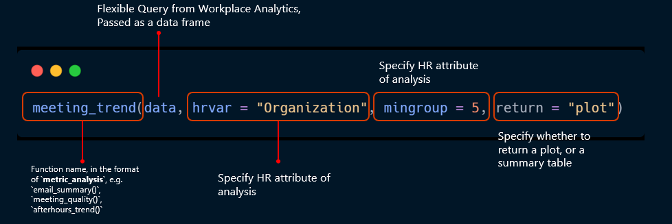
So far we have explored the hrvar and return arguments. We will use the mingroup in the next section.
Exporting plots and tables
Tables and plots can be saved with the export() function. This functions allows you to save plots and tables into your local drive.
One again, adding an additional forward-Pipe operator we can write:
sq_data %>%
    analysis_scope(hrvar = "Organization") %>%
    export()
Four steps from data to output
The examples above illustrate how the use of wpa can be summarized in 4 simple steps: Load the package, read-in query data, run functions and export results. The script below illustrates this functionality:
library(wpa) # Step 1

person_data <- import_wpa("myquery.csv") # Step 2

person_data %>% analysis_scope() # Step 3

person_data %>%
    analysis_scope() %>%
    export() # Step 4
Ready to learn more?
Let’s go to the Data Validation section to explore options for validating data. To skip straight to analysis, see the Summary Functions section.