Run a summary of Key Metrics without aggregation

Return a heatmapped table directly from the aggregated / summarised data. Unlike keymetrics_scan() which performs a person-level aggregation, there is no calculation for keymetrics_scan_asis() and the values are rendered as they are passed into the function.

keymetrics_scan_asis(
  data,
  row_var,
  col_var,
  group_var = col_var,
  value_var = "value",
  title = NULL,
  subtitle = NULL,
  caption = NULL,
  ylab = row_var,
  xlab = "Metrics",
  rounding = 1,
  low = rgb2hex(7, 111, 161),
  mid = rgb2hex(241, 204, 158),
  high = rgb2hex(216, 24, 42),
  textsize = 2
)

Arguments

data

data frame containing data to plot. It is recommended to provide data in a 'long' table format where one grouping column forms the rows, a second column forms the columns, and a third numeric columns forms the

row_var

String containing name of the grouping variable that will form the rows of the heatmapped table.

col_var

String containing name of the grouping variable that will form the columns of the heatmapped table.

group_var

String containing name of the grouping variable by which heatmapping would apply. Defaults to col_var.

value_var

String containing name of the value variable that will form the values of the heatmapped table. Defaults to "value".

title

Title of the plot.

subtitle

Subtitle of the plot.

caption

Caption of the plot.

ylab

Y-axis label for the plot (group axis)

xlab

X-axis label of the plot (bar axis).

rounding

Numeric value to specify number of digits to show in data labels

low

String specifying colour code to use for low-value metrics. Arguments are passed directly to ggplot2::scale_fill_gradient2().

mid

String specifying colour code to use for mid-value metrics. Arguments are passed directly to ggplot2::scale_fill_gradient2().

high

String specifying colour code to use for high-value metrics. Arguments are passed directly to ggplot2::scale_fill_gradient2().

textsize

A numeric value specifying the text size to show in the plot.

Value

ggplot object for a heatmap table.

Examples

library(dplyr)

# Compute summary table
out_df <-
  sq_data %>%
  group_by(Organization) %>%
  summarise(
    across(
      .cols = c(
        Workweek_span,
        Collaboration_hours
        ),
      .fns = ~median(., na.rm = TRUE)
      ),
      .groups = "drop"
    ) %>%
tidyr::pivot_longer(
  cols = c("Workweek_span", "Collaboration_hours"),
  names_to = "metrics"
)

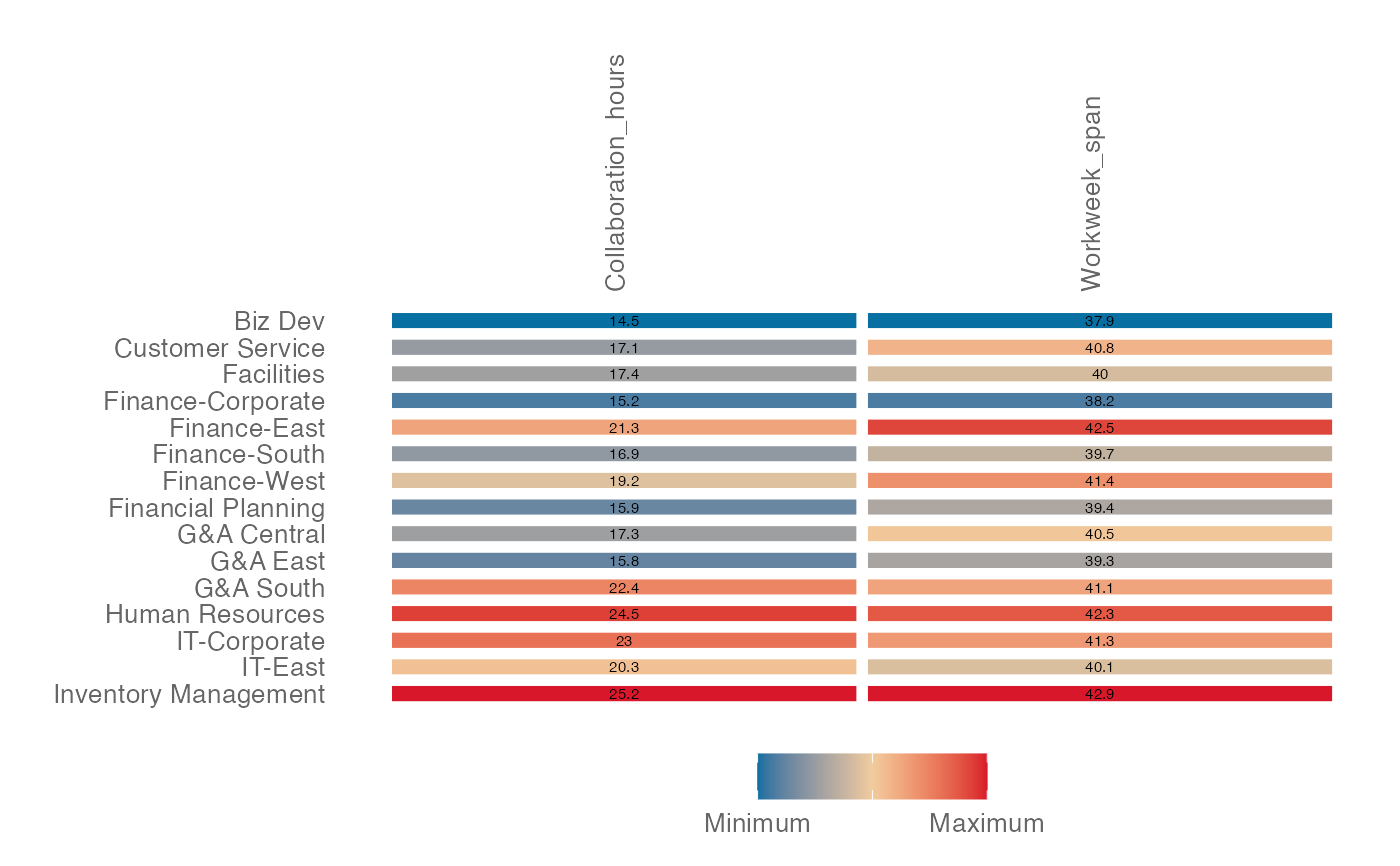
keymetrics_scan_asis(
  data = out_df,
  col_var = "metrics",
  row_var = "Organization"
)


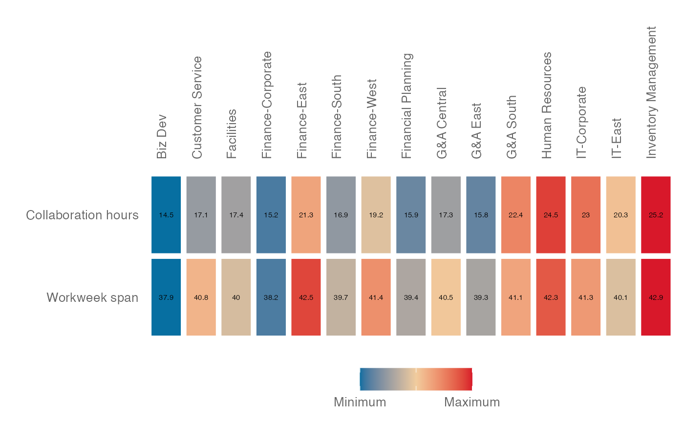# Show data the other way round
keymetrics_scan_asis(
  data = out_df,
  col_var = "Organization",
  row_var = "metrics",
  group_var = "metrics"
)