Summarise node centrality statistics with an igraph object

Pass an igraph object to the function and obtain centrality statistics for each node in the object as a data frame. This function works as a wrapper of the centralization functions in 'igraph'.

network_summary(graph, hrvar = NULL, return = "table")

Arguments

graph

'igraph' object that can be returned from network_g2g() or network_p2p()when the return argument is set to "network".

hrvar

String containing the name of the HR Variable by which to split metrics. Defaults to NULL.

return

String specifying what output to return. Valid inputs include:

"table"
"network"
"plot"

See Value for more information.

Value

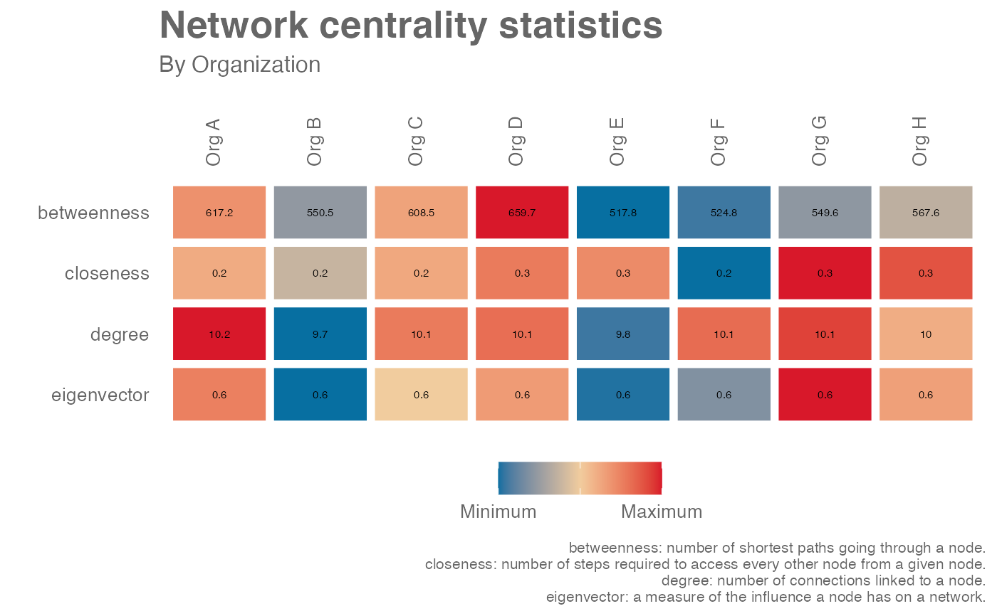
By default, a data frame containing centrality statistics. Available statistics include:

betweenness: number of shortest paths going through a node.
closeness: number of steps required to access every other node from a given node.
degree: number of connections linked to a node.
eigenvector: a measure of the influence a node has on a network. Please refer to the igraph package documentation for the detailed technical definition.

When "network" is passed to "return", an 'igraph' object is returned with additional node attributes containing centrality scores.

When "plot" is passed to "return", a summary table is returned showing the average centrality scores by HR attribute. This is currently available if there is a valid HR attribute.

Examples

# Simulate a p2p network
p2p_data <- p2p_data_sim()
g <- network_p2p(data = p2p_data, return = "network")

# Return summary table
network_summary(graph = g, return = "table")
#> # A tibble: 300 × 5
#>    node_id    betweenness closeness degree eigenvector
#>    <chr>            <dbl>     <dbl>  <dbl>       <dbl>
#>  1 SIM_ID_1           0       0.223     11       0.671
#>  2 SIM_ID_2          13.8     0.212     10       0.609
#>  3 SIM_ID_3          74.4     0.227     10       0.608
#>  4 SIM_ID_4         132.      0.229     10       0.578
#>  5 SIM_ID_6         333.      0.242     10       0.606
#>  6 SIM_ID_7         312.      0.233     10       0.564
#>  7 SIM_ID_236      1296.      0.234     11       0.956
#>  8 SIM_ID_9         326.      0.226     10       0.570
#>  9 SIM_ID_10        332.      0.221     10       0.560
#> 10 SIM_ID_11        235.      0.204     10       0.592
#> # … with 290 more rows

# Return network with node centrality statistics
network_summary(graph = g, return = "network")
#> IGRAPH 8df3483 DNW- 300 1500 -- 
#> + attr: weight (g/n), name (v/c), Organization (v/c), betweenness
#> | (v/n), closeness (v/n), degree (v/n), eigenvector (v/n), weight (e/n)
#> + edges from 8df3483 (vertex names):
#>  [1] SIM_ID_1->SIM_ID_2   SIM_ID_1->SIM_ID_3   SIM_ID_1->SIM_ID_4  
#>  [4] SIM_ID_1->SIM_ID_6   SIM_ID_1->SIM_ID_210 SIM_ID_1->SIM_ID_296
#>  [7] SIM_ID_1->SIM_ID_297 SIM_ID_1->SIM_ID_298 SIM_ID_1->SIM_ID_299
#> [10] SIM_ID_1->SIM_ID_5   SIM_ID_1->SIM_ID_300 SIM_ID_2->SIM_ID_3  
#> [13] SIM_ID_2->SIM_ID_4   SIM_ID_2->SIM_ID_7   SIM_ID_2->SIM_ID_287
#> [16] SIM_ID_2->SIM_ID_297 SIM_ID_2->SIM_ID_298 SIM_ID_2->SIM_ID_299
#> [19] SIM_ID_2->SIM_ID_5   SIM_ID_2->SIM_ID_300 SIM_ID_3->SIM_ID_4  
#> + ... omitted several edges

# Return summary plot
network_summary(graph = g, return = "plot", hrvar = "Organization")


# Simulate a g2g network and return table
g2 <- g2g_data %>% network_g2g(return = "network")
#> `time_investor` field not provided. Assuming `TimeInvestors_Organization` as the `time_investor` variable.
#> `collaborator` field not provided. Assuming `Collaborators_Organization` as the `collaborator` variable.
network_summary(graph = g2, return = "table")
#> # A tibble: 15 × 5
#>    node_id                 betweenness closeness degree eigenvector
#>    <chr>                         <dbl>     <dbl>  <dbl>       <dbl>
#>  1 "Biz\nDev"                    1.28      0.414      4       0.374
#>  2 "Customer\nService"           0         0.343      3       0.198
#>  3 "Facilities"                  1         0.444      4       0.517
#>  4 "Finance-Corporate"           0       NaN          2       0    
#>  5 "Finance-East"                8.83      0.571      6       0.847
#>  6 "Finance-South"              17.3       0.632      7       0.973
#>  7 "Finance-West"                4.67      0.522      5       0.715
#>  8 "Financial\nPlanning"         1.95      0.444      4       0.395
#>  9 "G&A\nCentral"                0       NaN          2       0    
#> 10 "G&A\nEast"                   0         0.387      3       0.269
#> 11 "G&A\nSouth"                 22.8       0.6        8       1    
#> 12 "Human\nResources"           12.6       0.5        6       0.735
#> 13 "IT-Corporate"                4.67      0.462      5       0.469
#> 14 "IT-East"                     0.417     0.429      4       0.490
#> 15 "Inventory\nManagement"      12.5       0.545      7       0.922

Summarise node centrality statistics with an igraph object

Arguments

Value

See also

Examples