Classify working pattern personas using a rule based algorithm

Apply a rule based algorithm to emails or instant messages sent by hour of day. Uses a binary week-based ('bw') method by default, with options to use the the person-average volume-based ('pav') method.

workpatterns_classify(
  data,
  hrvar = "Organization",
  values = "percent",
  signals = c("email", "IM"),
  start_hour = "0900",
  end_hour = "1700",
  exp_hours = NULL,
  mingroup = 5,
  active_threshold = 0,
  method = "bw",
  return = "plot"
)

Arguments

data

A data frame containing data from the Hourly Collaboration query.

hrvar

A string specifying the HR attribute to cut the data by. Defaults to NULL. This only affects the function when "table" is returned, and is only applicable for method = "bw".

values

Only valid if using pav method. Character vector to specify whether to return percentages or absolute values in "data" and "plot". Valid values are "percent" (default) and "abs".

signals

Character vector to specify which collaboration metrics to use:

• "email" (default) for emails only

• "IM" for Teams messages only

• "unscheduled_calls" for Unscheduled Calls only

• "meetings" for Meetings only

• or a combination of signals, such as c("email", "IM")

start_hour

A character vector specifying starting hours, e.g. "0900". Note that this currently only supports hourly increments. If the official hours specifying checking in and 9 AM and checking out at 5 PM, then "0900" should be supplied here.

end_hour

A character vector specifying starting hours, e.g. "1700". Note that this currently only supports hourly increments. If the official hours specifying checking in and 9 AM and checking out at 5 PM, then "1700" should be supplied here.

exp_hours

Numeric value representing the number of hours the population is expected to be active for throughout the workday. By default, this uses the difference between end_hour and start_hour. Only applicable with the 'bw' method.

mingroup

Numeric value setting the privacy threshold / minimum group size. Defaults to 5.

active_threshold

A numeric value specifying the minimum number of signals to be greater than in order to qualify as active. Defaults to 0. Only applicable for the binary-week method.

method

String to pass through specifying which method to use for classification. By default, a binary week-based (bw) method is used, with options to use the the person-average volume-based (pav) method.

return

String specifying what to return. This must be one of the following strings:

• "plot"

• "data"

• "table"

• "plot-area"

• "plot-hrvar" (only for bw method)

• "plot-dist" (only for bw method)

See Value for more information.

Value

Character vector to specify what to return. Valid options include:

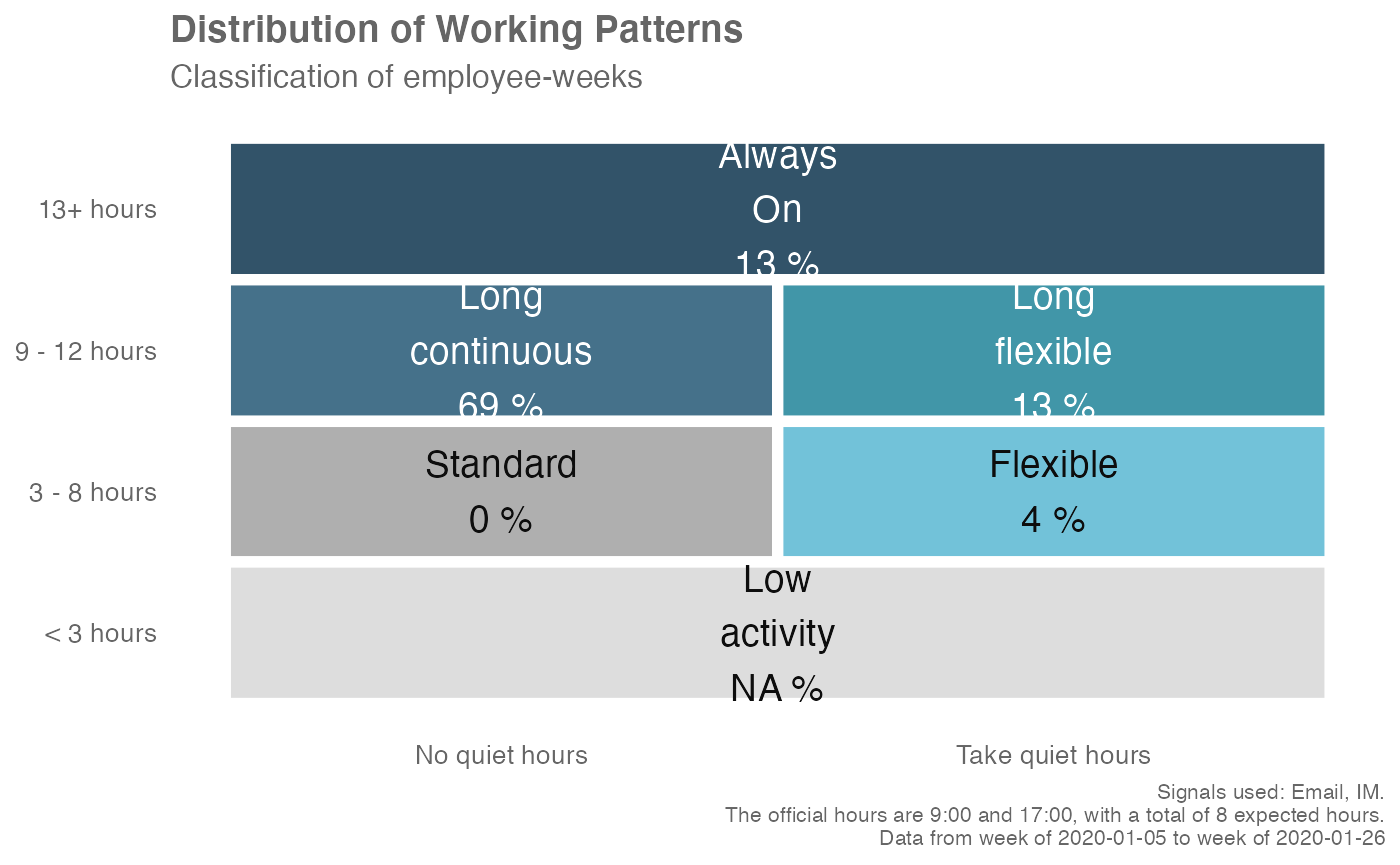
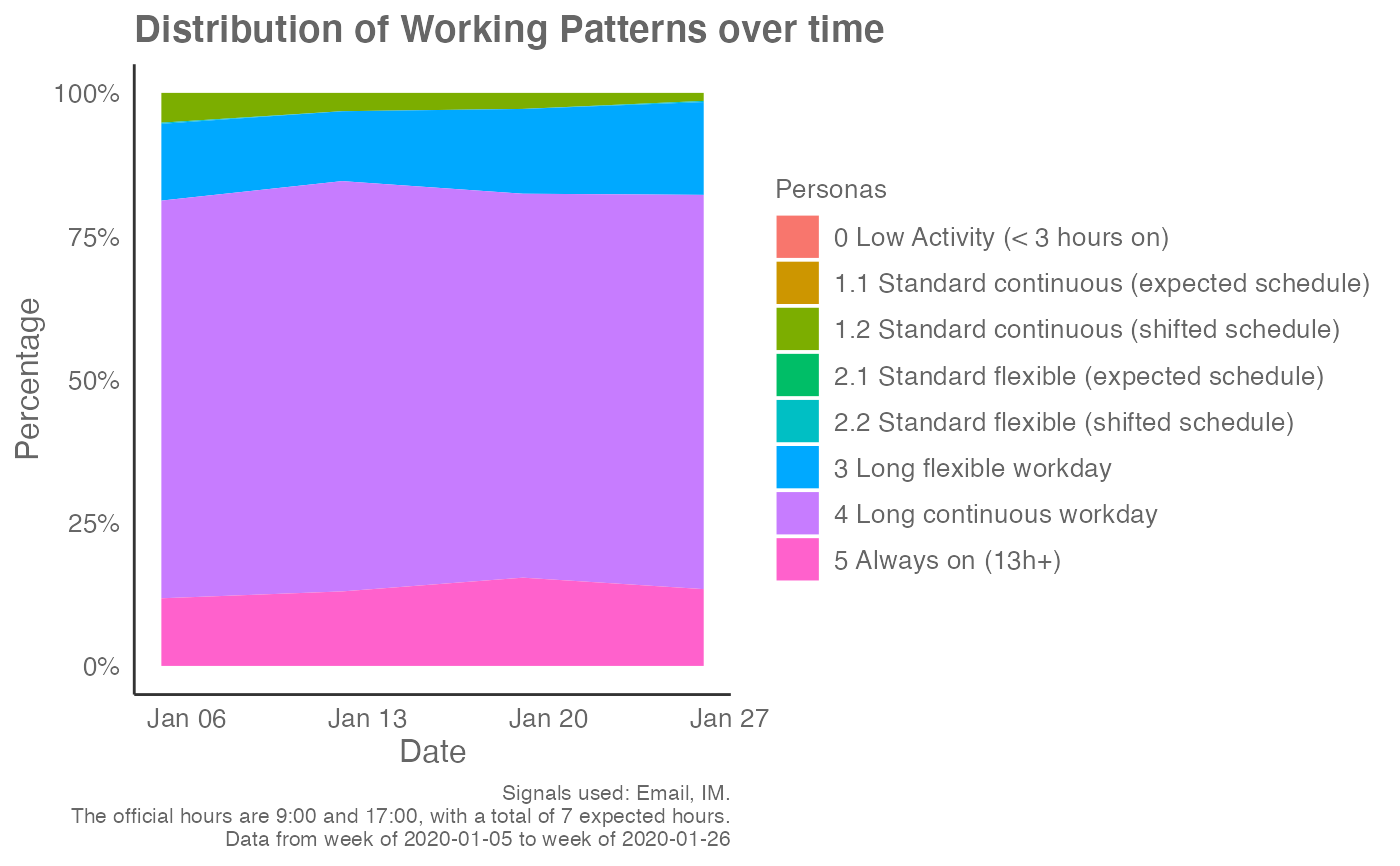
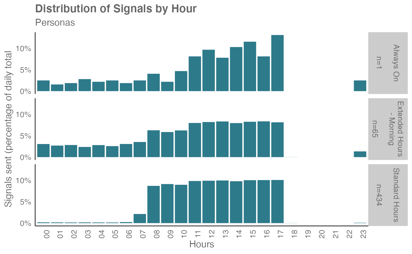
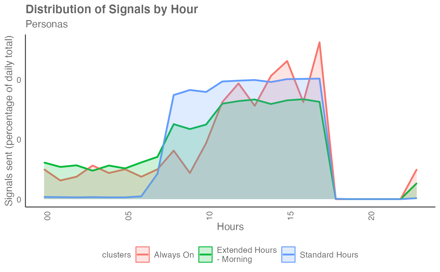
• "plot": ggplot object. With the bw method, this returns a grid showing the distribution of archetypes by 'breaks' and number of active hours (default). With the pav method, this returns a faceted bar plot which shows the percentage of signals sent in each hour, with each facet representing an archetype.

• "data": data frame. The raw data with the classified archetypes.

• "table": data frame. A summary table of the archetypes.

• "plot-area": ggplot object. With the bw method, this returns an area plot of the percentages of archetypes shown over time. With the pav method, this returns an area chart which shows the percentage of signals sent in each hour, with each line representing an archetype.

• "plot-hrvar": ggplot object. A bar plot showing the count of archetypes, faceted by the supplied HR attribute. This is only available for the bw method.

• "plot-dist": returns a heatmap plot of signal distribution by hour and archetypes. This is only available for the bw method.

Details

The working patterns archetypes are a set of segments created based on the aggregated hourly activity of employees. A motivation of creating these archetypes is to capture the diversity in working patterns, where for instance employees may choose to take multiple or extended breaks throughout the day, or choose to start or end earlier/later than their standard working hours. Two methods have been developed to capture the different working patterns.

This function is a wrapper around workpatterns_classify_bw() and workpatterns_classify_pav(), and calls each function depending on what is supplied to the method argument. Both methods implement a rule-based classification of either person-weeks or persons that pull apart different working patterns.

See individual sections below for details on the two different implementations.

Binary Week method

This method classifies each person-week into one of the eight archetypes:

• 0 Low Activity (< 3 hours on): fewer than 3 hours of active hours

• 1.1 Standard continuous (expected schedule): active hours equal to expected hours, with all activity confined within the expected start and end time

• 1.2 Standard continuous (shifted schedule): active hours equal to expected hours, with activity occurring beyond either the expected start or end time.

• 2.1 Standard flexible (expected schedule): active hours less than or equal to expected hours, with all activity confined within the expected start and end time

• 2.2 Standard flexible (shifted schedule): active hours less than or equal to expected hours, with activity occurring beyond either the expected start or end time.

• 3 Long flexible workday: number of active hours exceed expected hours, with breaks occurring throughout

• 4 Long continuous workday: number of active hours exceed expected hours, with activity happening in a continuous block (no breaks)

• 5 Always on (13h+): number of active hours greater than or equal to 13

Standard here denotes the behaviour of not exhibiting total number of active hours which exceed the expected total number of hours, as supplied by exp_hours. Continuous refers to the behaviour of not taking breaks, i.e. no inactive hours between the first and last active hours of the day, where flexible refers to the contrary.

This is the recommended method over pav for several reasons:

1. bw ignores volume effects, where activity volume can still bias the results towards the 'standard working hours'.

2. It captures the intuition that each individual can have 'light' and 'heavy' weeks with respect to workload.

The notion of 'breaks' in the 'binary-week' method is best understood as 'recurring disconnection time'. This denotes an hourly block where there is consistently no activity occurring throughout the week. Note that this applies a stricter criterion compared to the common definition of a break, which is simply a time interval where no active work is being done, and thus the more specific terminology 'recurring disconnection time' is preferred.

In the standard plot output, the archetypes have been abbreviated to show the following:

• Low Activity - archetype 0

• Standard - archetypes 1.1 and 1.2

• Flexible - archetypes 2.1 and 2.2

• Long continuous - archetype 4

• Long flexible - archetype 3

• Always On - archetype 5

Person Average method

This method classifies each person (based on unique PersonId) into one of the six archetypes:

• Absent: Fewer than 10 signals over the week.

• Extended Hours - Morning: 15%+ of collaboration before start hours and less than 70% within standard hours, and less than 15% of collaboration after end hours

• Extended Hours - Evening: Less than 15% of collaboration before start hours and less than 70% within standard hours, and 15%+ of collaboration after end hours

• Overnight workers: less than 30% of collaboration happens within standard hours

• Standard Hours: over 70% of collaboration within standard hours

• Always On: over 15% of collaboration happens before starting hour and end hour (both conditions must satisfy) and less than 70% of collaboration within standard hours

Flexibility Index

The Working Patterns archetypes as calculated using the binary-week method shares many similarities with the Flexibility Index (see flex_index()):

• Both are computed directly from the Hourly Collaboration Flexible Query.

• Both apply the same binary conversion of activity on the signals from the Hourly Collaboration Flexible Query.

See also

Other Clustering: personas_hclust(), workpatterns_hclust()

Other Working Patterns: flex_index(), identify_shifts_wp(), identify_shifts(), plot_flex_index(), workpatterns_area(), workpatterns_classify_bw(), workpatterns_classify_pav(), workpatterns_hclust(), workpatterns_rank(), workpatterns_report()

Author

Ainize Cidoncha ainize.cidoncha@microsoft.com

Carlos Morales Torrado carlos.morales@microsoft.com

Martin Chan martin.chan@microsoft.com

Examples

# Returns a plot by default
em_data %>% workpatterns_classify(method = "bw")


# Return an area plot
# With custom expected hours
em_data %>%
  workpatterns_classify(
    method = "bw",
    return = "plot-area",
    exp_hours = 7
      )


# \donttest{

em_data %>% workpatterns_classify(method = "bw", return = "table")
#> # A tibble: 5 × 17
#>   Personas      Biz De…¹ Custo…² Facil…³ Finan…⁴ Finan…⁵ Finan…⁶ Finan…⁷ Finan…⁸
#>   <fct>            <dbl>   <dbl>   <dbl>   <dbl>   <dbl>   <dbl>   <dbl>   <dbl>
#> 1 1.2 Standard… NA       NA      0.00806 NA      NA       0.0132 NA      NA     
#> 2 2.2 Standard… NA       NA      0.105    0.0735  0.0515  0.112   0.0417 NA     
#> 3 3 Long flexi…  0.111    0.0938 0.0565   0.0956  0.110   0.125   0.0417  0.0463
#> 4 4 Long conti…  0.880    0.885  0.758    0.75    0.632   0.599   0.817   0.907 
#> 5 5 Always on …  0.00926  0.0208 0.0726   0.0809  0.206   0.151   0.1     0.0463
#> # … with 8 more variables: `G&A Central` <dbl>, `G&A East` <dbl>,
#> #   `G&A South` <dbl>, `Human Resources` <dbl>, `IT-Corporate` <dbl>,
#> #   `IT-East` <dbl>, `Inventory Management` <dbl>, Total <dbl>, and abbreviated
#> #   variable names ¹​`Biz Dev`, ²​`Customer Service`, ³​Facilities,
#> #   ⁴​`Finance-Corporate`, ⁵​`Finance-East`, ⁶​`Finance-South`, ⁷​`Finance-West`,
#> #   ⁸​`Financial Planning`

em_data %>% workpatterns_classify(method = "pav")


em_data %>% workpatterns_classify(method = "pav", return = "plot-area")


# }