Distribution of After-hours Collaboration Hours as a 100% stacked bar
Source:R/afterhours_dist.R
afterhours_dist.RdAnalyse the distribution of weekly after-hours collaboration time. Returns a stacked bar plot by default. Additional options available to return a table with distribution elements.
afterhours_dist(
  data,
  hrvar = "Organization",
  mingroup = 5,
  return = "plot",
  cut = c(1, 2, 3)
)
Arguments
- data
A Standard Person Query dataset in the form of a data frame.
- hrvar
String containing the name of the HR Variable by which to split metrics. Defaults to
"Organization". To run the analysis on the total instead of splitting by an HR attribute, supplyNULL(without quotes).- mingroup
Numeric value setting the privacy threshold / minimum group size. Defaults to 5.
- return
String specifying what to return. This must be one of the following strings:
"plot""table"
See
Valuefor more information.- cut
A vector specifying the cuts to use for the data, accepting "default" or "range-cut" as character vector, or a numeric value of length three to specify the exact breaks to use. e.g. c(1, 3, 5)
Value
A different output is returned depending on the value passed to the return argument:
"plot": 'ggplot' object. A stacked bar plot for the metric."table": data frame. A summary table for the metric.
Details
Uses the metric After_hours_collaboration_hours.
See create_dist() for applying the same analysis to a different metric.
See also
Other Visualization:
afterhours_fizz(),
afterhours_line(),
afterhours_rank(),
afterhours_summary(),
afterhours_trend(),
collaboration_area(),
collaboration_dist(),
collaboration_fizz(),
collaboration_line(),
collaboration_rank(),
collaboration_sum(),
collaboration_trend(),
create_bar(),
create_bar_asis(),
create_boxplot(),
create_bubble(),
create_dist(),
create_fizz(),
create_inc(),
create_line(),
create_line_asis(),
create_period_scatter(),
create_rank(),
create_sankey(),
create_scatter(),
create_stacked(),
create_tracking(),
create_trend(),
email_dist(),
email_fizz(),
email_line(),
email_rank(),
email_summary(),
email_trend(),
external_dist(),
external_fizz(),
external_line(),
external_network_plot(),
external_rank(),
external_sum(),
hr_trend(),
hrvar_count(),
hrvar_trend(),
internal_network_plot(),
keymetrics_scan(),
meeting_dist(),
meeting_fizz(),
meeting_line(),
meeting_quality(),
meeting_rank(),
meeting_summary(),
meeting_trend(),
meetingtype_dist(),
meetingtype_dist_ca(),
meetingtype_dist_mt(),
meetingtype_summary(),
mgrcoatt_dist(),
mgrrel_matrix(),
one2one_dist(),
one2one_fizz(),
one2one_freq(),
one2one_line(),
one2one_rank(),
one2one_sum(),
one2one_trend(),
period_change(),
workloads_dist(),
workloads_fizz(),
workloads_line(),
workloads_rank(),
workloads_summary(),
workloads_trend(),
workpatterns_area(),
workpatterns_rank()
Other After-hours Collaboration:
afterhours_fizz(),
afterhours_line(),
afterhours_rank(),
afterhours_summary(),
afterhours_trend(),
external_rank()
Examples
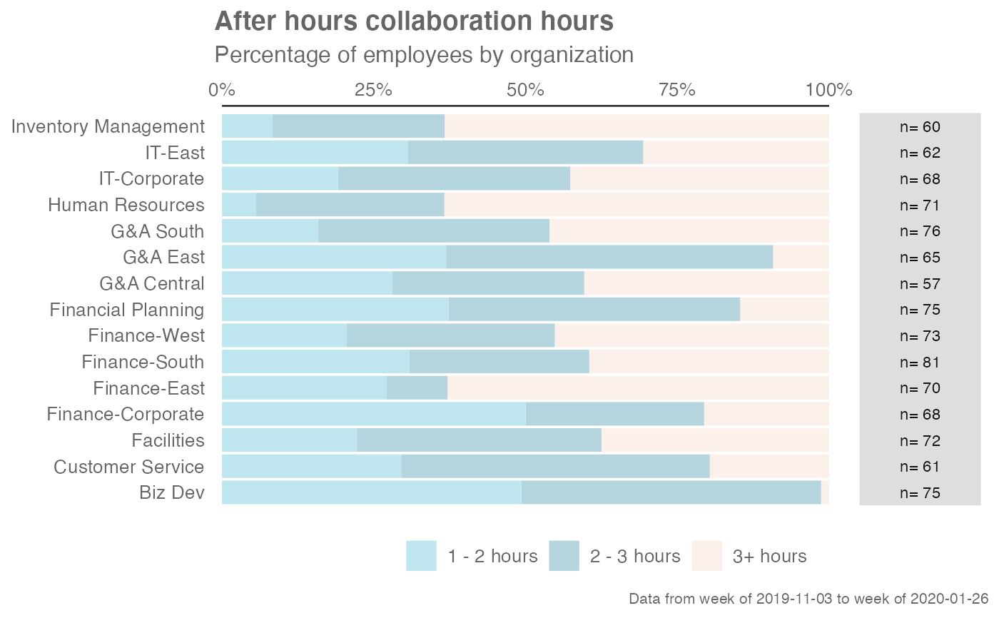
# Return plot
afterhours_dist(sq_data, hrvar = "Organization")
 # Return summary table
afterhours_dist(sq_data, hrvar = "Organization", return = "table")
#> # A tibble: 5 × 5
#> group `1 - 2 hours` `2 - 3 hours` `3+ hours` Employee_Count
#> <fct> <dbl> <dbl> <dbl> <int>
#> 1 Customer Service 0.246 0.492 0.262 61
#> 2 Finance 0.325 0.25 0.425 292
#> 3 Financial Planning 0.44 0.36 0.2 75
#> 4 Human Resources 0.0986 0.254 0.648 71
#> 5 IT 0.238 0.377 0.385 130
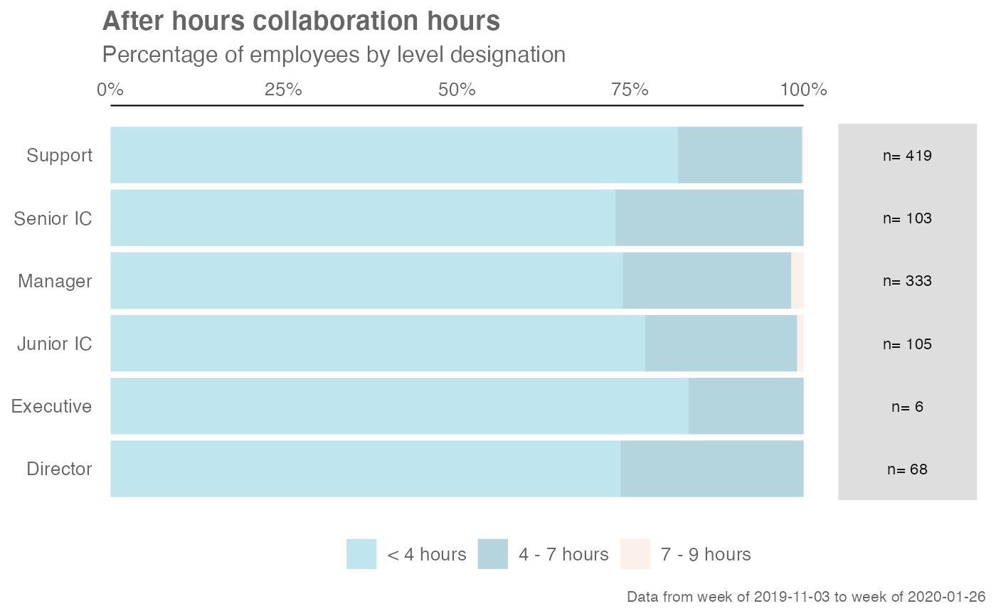
# Return result with a custom specified breaks
afterhours_dist(sq_data, hrvar = "LevelDesignation", cut = c(4, 7, 9))
# Return summary table
afterhours_dist(sq_data, hrvar = "Organization", return = "table")
#> # A tibble: 5 × 5
#> group `1 - 2 hours` `2 - 3 hours` `3+ hours` Employee_Count
#> <fct> <dbl> <dbl> <dbl> <int>
#> 1 Customer Service 0.246 0.492 0.262 61
#> 2 Finance 0.325 0.25 0.425 292
#> 3 Financial Planning 0.44 0.36 0.2 75
#> 4 Human Resources 0.0986 0.254 0.648 71
#> 5 IT 0.238 0.377 0.385 130
# Return result with a custom specified breaks
afterhours_dist(sq_data, hrvar = "LevelDesignation", cut = c(4, 7, 9))