Provides an overview analysis of Weekly Digital Collaboration. Returns an stacked area plot of Email and Meeting Hours by default. Additional options available to return a summary table.
collaboration_area(data, hrvar = NULL, mingroup = 5, return = "plot")

collab_area(data, hrvar = NULL, mingroup = 5, return = "plot")
Arguments
- data
A Standard Person Query dataset in the form of a data frame. A Ways of Working assessment dataset may also be provided, in which Unscheduled call hours would be included in the output.
- hrvar
HR Variable by which to split metrics, defaults to
NULL, but accepts any character vector, e.g. "LevelDesignation". IfNULLis passed, the organizational attribute is automatically populated as "Total".- mingroup
Numeric value setting the privacy threshold / minimum group size. Defaults to 5.
- return
String specifying what to return. This must be one of the following strings:
"plot""table"
See
Valuefor more information.
Value
A different output is returned depending on the value passed to the return argument:
"plot": 'ggplot' object. A stacked area plot for the metric."table": data frame. A summary table for the metric.
Details
Uses the metrics Meeting_hours, Email_hours, Unscheduled_Call_hours,
and Instant_Message_hours.
See also
Other Visualization:
afterhours_dist(),
afterhours_fizz(),
afterhours_line(),
afterhours_rank(),
afterhours_summary(),
afterhours_trend(),
collaboration_dist(),
collaboration_fizz(),
collaboration_line(),
collaboration_rank(),
collaboration_sum(),
collaboration_trend(),
create_bar(),
create_bar_asis(),
create_boxplot(),
create_bubble(),
create_dist(),
create_fizz(),
create_inc(),
create_line(),
create_line_asis(),
create_period_scatter(),
create_rank(),
create_sankey(),
create_scatter(),
create_stacked(),
create_tracking(),
create_trend(),
email_dist(),
email_fizz(),
email_line(),
email_rank(),
email_summary(),
email_trend(),
external_dist(),
external_fizz(),
external_line(),
external_network_plot(),
external_rank(),
external_sum(),
hr_trend(),
hrvar_count(),
hrvar_trend(),
internal_network_plot(),
keymetrics_scan(),
meeting_dist(),
meeting_fizz(),
meeting_line(),
meeting_quality(),
meeting_rank(),
meeting_summary(),
meeting_trend(),
meetingtype_dist(),
meetingtype_dist_ca(),
meetingtype_dist_mt(),
meetingtype_summary(),
mgrcoatt_dist(),
mgrrel_matrix(),
one2one_dist(),
one2one_fizz(),
one2one_freq(),
one2one_line(),
one2one_rank(),
one2one_sum(),
one2one_trend(),
period_change(),
workloads_dist(),
workloads_fizz(),
workloads_line(),
workloads_rank(),
workloads_summary(),
workloads_trend(),
workpatterns_area(),
workpatterns_rank()
Other Collaboration:
collaboration_dist(),
collaboration_fizz(),
collaboration_line(),
collaboration_rank(),
collaboration_sum(),
collaboration_trend()
Examples
# \donttest{
# Return plot with total (default)
collaboration_area(sq_data)
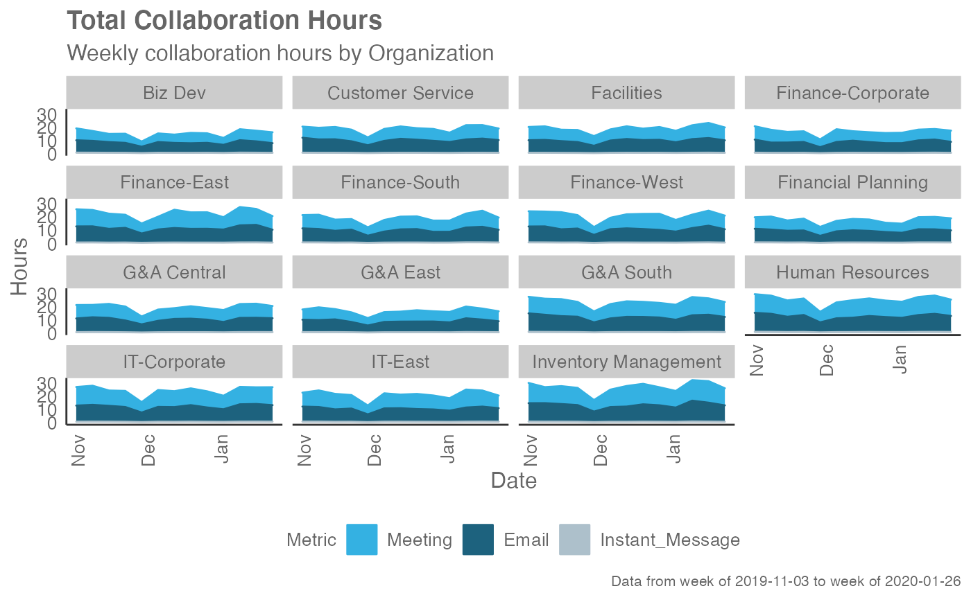
 # Return plot with hrvar split
collaboration_area(sq_data, hrvar = "Organization")
# Return plot with hrvar split
collaboration_area(sq_data, hrvar = "Organization")
 # Return summary table
collaboration_area(sq_data, return = "table")
#> # A tibble: 7 × 7
#> Date group Meeting_hours Email_hours Instant_Message_hours
#> <date> <chr> <dbl> <dbl> <dbl>
#> 1 2019-12-15 Total 10.5 10.3 0.615
#> 2 2019-12-22 Total 10.6 10.2 0.610
#> 3 2019-12-29 Total 10.2 9.30 0.564
#> 4 2020-01-05 Total 8.91 8.67 0.532
#> 5 2020-01-12 Total 11.4 11.2 0.677
#> 6 2020-01-19 Total 11.3 11.8 0.712
#> 7 2020-01-26 Total 10.2 10.1 0.612
#> # ℹ 2 more variables: Employee_Count <int>, Collaboration_hours <dbl>
# }
# Return summary table
collaboration_area(sq_data, return = "table")
#> # A tibble: 7 × 7
#> Date group Meeting_hours Email_hours Instant_Message_hours
#> <date> <chr> <dbl> <dbl> <dbl>
#> 1 2019-12-15 Total 10.5 10.3 0.615
#> 2 2019-12-22 Total 10.6 10.2 0.610
#> 3 2019-12-29 Total 10.2 9.30 0.564
#> 4 2020-01-05 Total 8.91 8.67 0.532
#> 5 2020-01-12 Total 11.4 11.2 0.677
#> 6 2020-01-19 Total 11.3 11.8 0.712
#> 7 2020-01-26 Total 10.2 10.1 0.612
#> # ℹ 2 more variables: Employee_Count <int>, Collaboration_hours <dbl>
# }