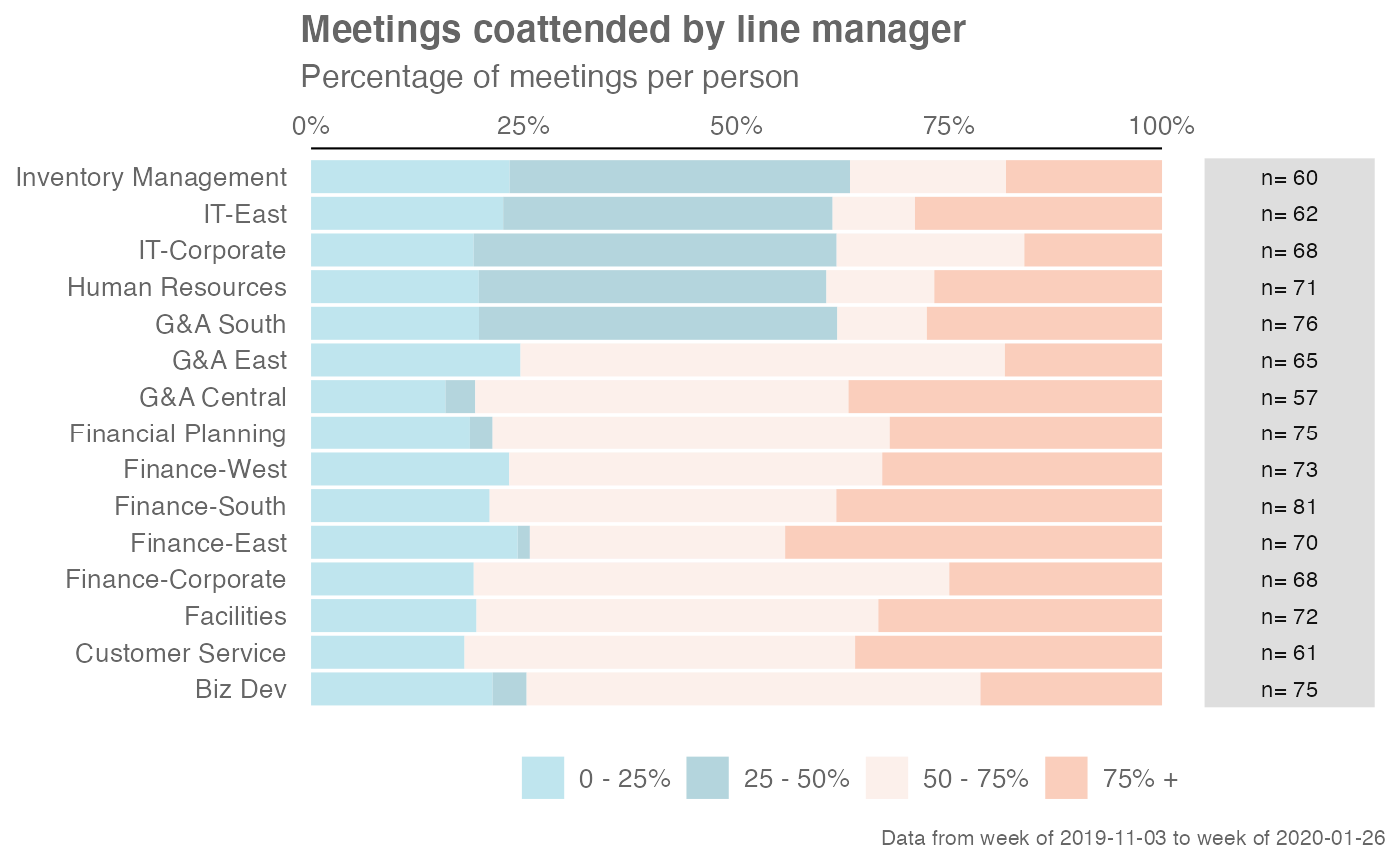
Analyze degree of attendance between employes and their managers. Returns a stacked bar plot of different buckets of coattendance. Additional options available to return a table with distribution elements.
mgrcoatt_dist(data, hrvar = "Organization", mingroup = 5, return = "plot")Arguments
- data
A Standard Person Query dataset in the form of a data frame.
- hrvar
String containing the name of the HR Variable by which to split metrics. Defaults to
"Organization". To run the analysis on the total instead of splitting by an HR attribute, supplyNULL(without quotes).- mingroup
Numeric value setting the privacy threshold / minimum group size. Defaults to 5.
- return
String specifying what to return. This must be one of the following strings:
"plot""table"
See
Valuefor more information.
Value
A different output is returned depending on the value passed to the return
argument:
"plot": ggplot object. A stacked bar plot showing the distribution of manager co-attendance time."table": data frame. A summary table for manager co-attendance time.
See also
Other Visualization:
afterhours_dist(),
afterhours_fizz(),
afterhours_line(),
afterhours_rank(),
afterhours_summary(),
afterhours_trend(),
collaboration_area(),
collaboration_dist(),
collaboration_fizz(),
collaboration_line(),
collaboration_rank(),
collaboration_sum(),
collaboration_trend(),
create_bar(),
create_bar_asis(),
create_boxplot(),
create_bubble(),
create_dist(),
create_fizz(),
create_inc(),
create_line(),
create_line_asis(),
create_period_scatter(),
create_rank(),
create_sankey(),
create_scatter(),
create_stacked(),
create_tracking(),
create_trend(),
email_dist(),
email_fizz(),
email_line(),
email_rank(),
email_summary(),
email_trend(),
external_dist(),
external_fizz(),
external_line(),
external_network_plot(),
external_rank(),
external_sum(),
hr_trend(),
hrvar_count(),
hrvar_trend(),
internal_network_plot(),
keymetrics_scan(),
meeting_dist(),
meeting_fizz(),
meeting_line(),
meeting_quality(),
meeting_rank(),
meeting_summary(),
meeting_trend(),
meetingtype_dist(),
meetingtype_dist_ca(),
meetingtype_dist_mt(),
meetingtype_summary(),
mgrrel_matrix(),
one2one_dist(),
one2one_fizz(),
one2one_freq(),
one2one_line(),
one2one_rank(),
one2one_sum(),
one2one_trend(),
period_change(),
workloads_dist(),
workloads_fizz(),
workloads_line(),
workloads_rank(),
workloads_summary(),
workloads_trend(),
workpatterns_area(),
workpatterns_rank()
Other Managerial Relations:
mgrrel_matrix(),
one2one_dist(),
one2one_fizz(),
one2one_freq(),
one2one_line(),
one2one_rank(),
one2one_sum(),
one2one_trend()
Examples
# Return plot
mgrcoatt_dist(sq_data, hrvar = "Organization", return = "plot")


# Return summary table
mgrcoatt_dist(sq_data, hrvar = "Organization", return = "table")
#> # A tibble: 5 × 5
#>   group              `0 - 25%` `25 - 50%` `50 - 75%` `75% +`
#>   <chr>                  <dbl>      <dbl>      <dbl>   <dbl>
#> 1 Customer Service       0.180     0.0492      0.443   0.328
#> 2 Finance                0.219     0.0240      0.428   0.329
#> 3 Financial Planning     0.187     0.0667      0.467   0.28
#> 4 Human Resources        0.211     0.380       0.155   0.254
#> 5 IT                     0.215     0.377       0.192   0.215
# Return summary table
mgrcoatt_dist(sq_data, hrvar = "Organization", return = "table")
#> # A tibble: 5 × 5
#> group `0 - 25%` `25 - 50%` `50 - 75%` `75% +`
#> <chr> <dbl> <dbl> <dbl> <dbl>
#> 1 Customer Service 0.180 0.0492 0.443 0.328
#> 2 Finance 0.219 0.0240 0.428 0.329
#> 3 Financial Planning 0.187 0.0667 0.467 0.28
#> 4 Human Resources 0.211 0.380 0.155 0.254
#> 5 IT 0.215 0.377 0.192 0.215