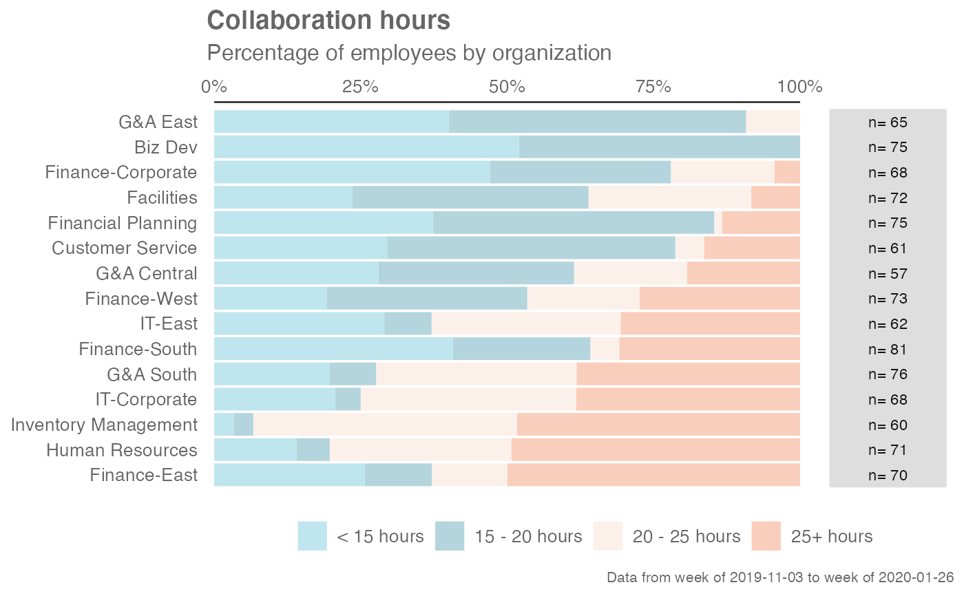
Horizontal 100 percent stacked bar plot for any metric

Provides an analysis of the distribution of a selected metric. Returns a stacked bar plot by default. Additional options available to return a table with distribution elements.

create_dist(
  data,
  metric,
  hrvar = "Organization",
  mingroup = 5,
  return = "plot",
  cut = c(15, 20, 25),
  dist_colours = c("#facebc", "#fcf0eb", "#b4d5dd", "#bfe5ee"),
  unit = "hours",
  lbound = 0,
  ubound = 100,
  sort_by = NULL,
  labels = NULL
)

Arguments

data

A Standard Person Query dataset in the form of a data frame.

metric

String containing the name of the metric, e.g. "Collaboration_hours"

hrvar

String containing the name of the HR Variable by which to split metrics. Defaults to "Organization". To run the analysis on the total instead of splitting by an HR attribute, supply NULL (without quotes).

mingroup

Numeric value setting the privacy threshold / minimum group size. Defaults to 5.

return

String specifying what to return. This must be one of the following strings:

"plot"
"table"

See Value for more information.

cut

A numeric vector of length three to specify the breaks for the distribution, e.g. c(10, 15, 20)

dist_colours

A character vector of length four to specify colour codes for the stacked bars.

unit

String to specify what unit to use. This defaults to "hours" but can accept any custom string. See cut_hour() for more details.

lbound

Numeric. Specifies the lower bound (inclusive) value for the minimum label. Defaults to 0.

ubound

Numeric. Specifies the upper bound (inclusive) value for the maximum label. Defaults to 100.

sort_by

String to specify the bucket label to sort by. Defaults to NULL (no sorting).

labels

Character vector to override labels for the created categorical variables. Must be a named vector - see examples.

Value

A different output is returned depending on the value passed to the return argument:

"plot": 'ggplot' object. A stacked bar plot for the metric.
"table": data frame. A summary table for the metric.

Other Visualization: afterhours_dist(), afterhours_fizz(), afterhours_line(), afterhours_rank(), afterhours_summary(), afterhours_trend(), collaboration_area(), collaboration_dist(), collaboration_fizz(), collaboration_line(), collaboration_rank(), collaboration_sum(), collaboration_trend(), create_bar_asis(), create_bar(), create_boxplot(), create_bubble(), create_fizz(), create_inc(), create_line_asis(), create_line(), create_period_scatter(), create_rank(), create_sankey(), create_scatter(), create_stacked(), create_tracking(), create_trend(), email_dist(), email_fizz(), email_line(), email_rank(), email_summary(), email_trend(), external_dist(), external_fizz(), external_line(), external_network_plot(), external_rank(), external_sum(), hr_trend(), hrvar_count(), hrvar_trend(), internal_network_plot(), keymetrics_scan(), meeting_dist(), meeting_fizz(), meeting_line(), meeting_quality(), meeting_rank(), meeting_summary(), meeting_trend(), meetingtype_dist_ca(), meetingtype_dist_mt(), meetingtype_dist(), meetingtype_summary(), mgrcoatt_dist(), mgrrel_matrix(), one2one_dist(), one2one_fizz(), one2one_freq(), one2one_line(), one2one_rank(), one2one_sum(), one2one_trend(), period_change(), workloads_dist(), workloads_fizz(), workloads_line(), workloads_rank(), workloads_summary(), workloads_trend(), workpatterns_area(), workpatterns_rank()

Other Flexible: create_bar_asis(), create_bar(), create_boxplot(), create_bubble(), create_density(), create_fizz(), create_hist(), create_inc(), create_line_asis(), create_line(), create_period_scatter(), create_rank(), create_sankey(), create_scatter(), create_stacked(), create_tracking(), create_trend(), period_change()

Examples

# Return plot
create_dist(sq_data, metric = "Collaboration_hours", hrvar = "Organization")


# Return summary table
create_dist(sq_data, metric = "Collaboration_hours", hrvar = "Organization", return = "table")
#> # A tibble: 15 × 6
#>    group                `< 15 hours` `15 - 20 hours` 20 - 25 h…¹ 25+ h…² Emplo…³
#>    <fct>                       <dbl>           <dbl>       <dbl>   <dbl>   <int>
#>  1 Biz Dev                    0.52            0.48       NA      NA           75
#>  2 Customer Service           0.295           0.492       0.0492  0.164       61
#>  3 Facilities                 0.236           0.403       0.278   0.0833      72
#>  4 Finance-Corporate          0.471           0.309       0.176   0.0441      68
#>  5 Finance-East               0.257           0.114       0.129   0.5         70
#>  6 Finance-South              0.407           0.235       0.0494  0.309       81
#>  7 Finance-West               0.192           0.342       0.192   0.274       73
#>  8 Financial Planning         0.373           0.48        0.0133  0.133       75
#>  9 G&A Central                0.281           0.333       0.193   0.193       57
#> 10 G&A East                   0.4             0.508       0.0923 NA           65
#> 11 G&A South                  0.197           0.0789      0.342   0.382       76
#> 12 Human Resources            0.141           0.0563      0.310   0.493       71
#> 13 IT-Corporate               0.206           0.0441      0.368   0.382       68
#> 14 IT-East                    0.290           0.0806      0.323   0.306       62
#> 15 Inventory Management       0.0333          0.0333      0.45    0.483       60
#> # … with abbreviated variable names ¹`20 - 25 hours`, ²`25+ hours`,
#> #   ³Employee_Count

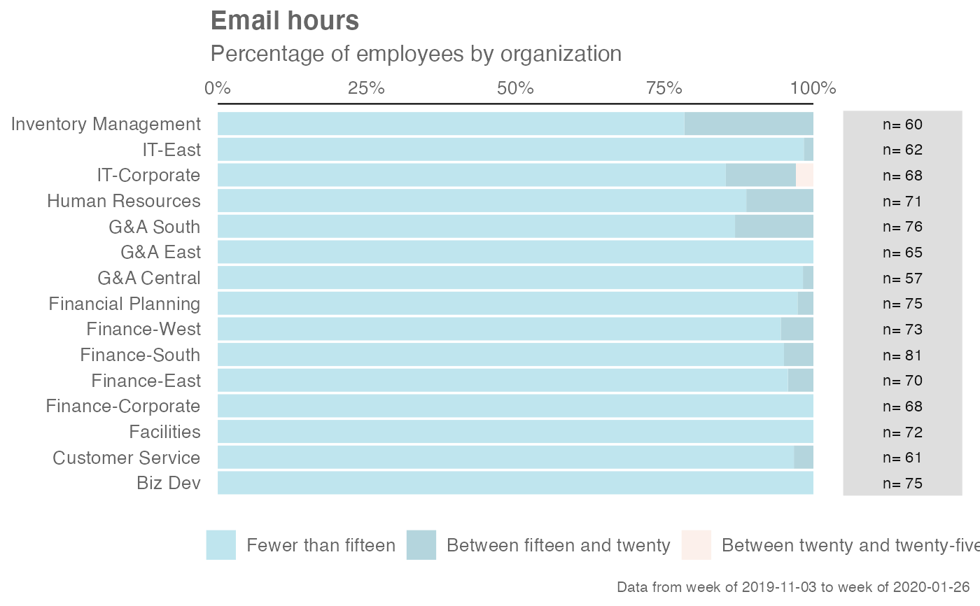
# Use custom labels by providing a label vector
eh_labels <- c(
  "Fewer than fifteen" = "< 15 hours",
  "Between fifteen and twenty" = "15 - 20 hours",
  "Between twenty and twenty-five" = "20 - 25 hours",
  "More than twenty-five" = "25+ hours"
)

sq_data %>%
  create_dist(metric = "Email_hours",
              labels = eh_labels, return = "plot")


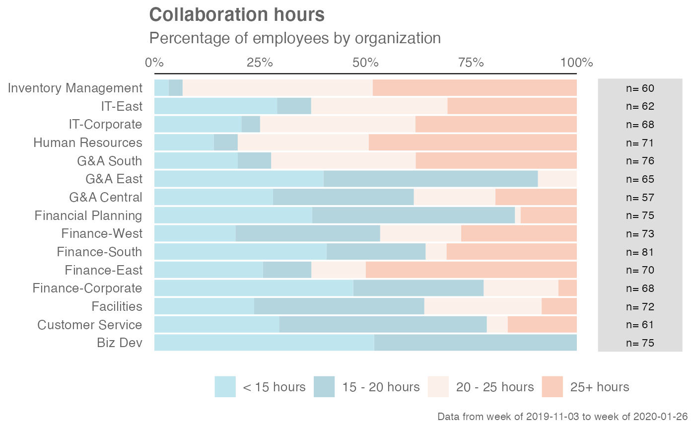
# Sort by a category
sq_data %>%
  create_dist(metric = "Collaboration_hours",
              sort_by = "25+ hours")

Horizontal 100 percent stacked bar plot for any metric

Arguments

Value

See also

Examples