Rank all groups across HR attributes on a selected Viva Insights metric
Source:R/create_rank.R
create_rank.RdThis function scans a standard Person query output for groups with high levels of a given Viva Insights Metric. Returns a plot by default, with an option to return a table with all groups (across multiple HR attributes) ranked by the specified metric.
create_rank(
  data,
  metric,
  hrvar = extract_hr(data, exclude_constants = TRUE),
  mingroup = 5,
  return = "table",
  mode = "simple",
  plot_mode = 1
)
Arguments
- data
A Standard Person Query dataset in the form of a data frame.
- metric
Character string containing the name of the metric, e.g. "Collaboration_hours"
- hrvar
String containing the name of the HR Variable by which to split metrics. Defaults to
"Organization". To run the analysis on the total instead of splitting by an HR attribute, supplyNULL(without quotes).- mingroup
Numeric value setting the privacy threshold / minimum group size. Defaults to 5.
- return
String specifying what to return. This must be one of the following strings:
"plot"(default)"table"
See
Valuefor more information.- mode
String to specify calculation mode. Must be either:
"simple""combine"
- plot_mode
Numeric vector to determine which plot mode to return. Must be either
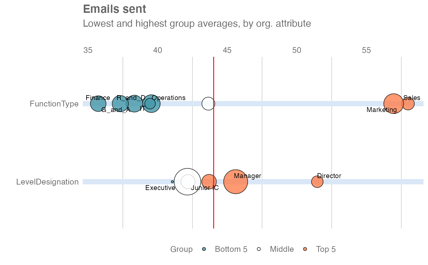
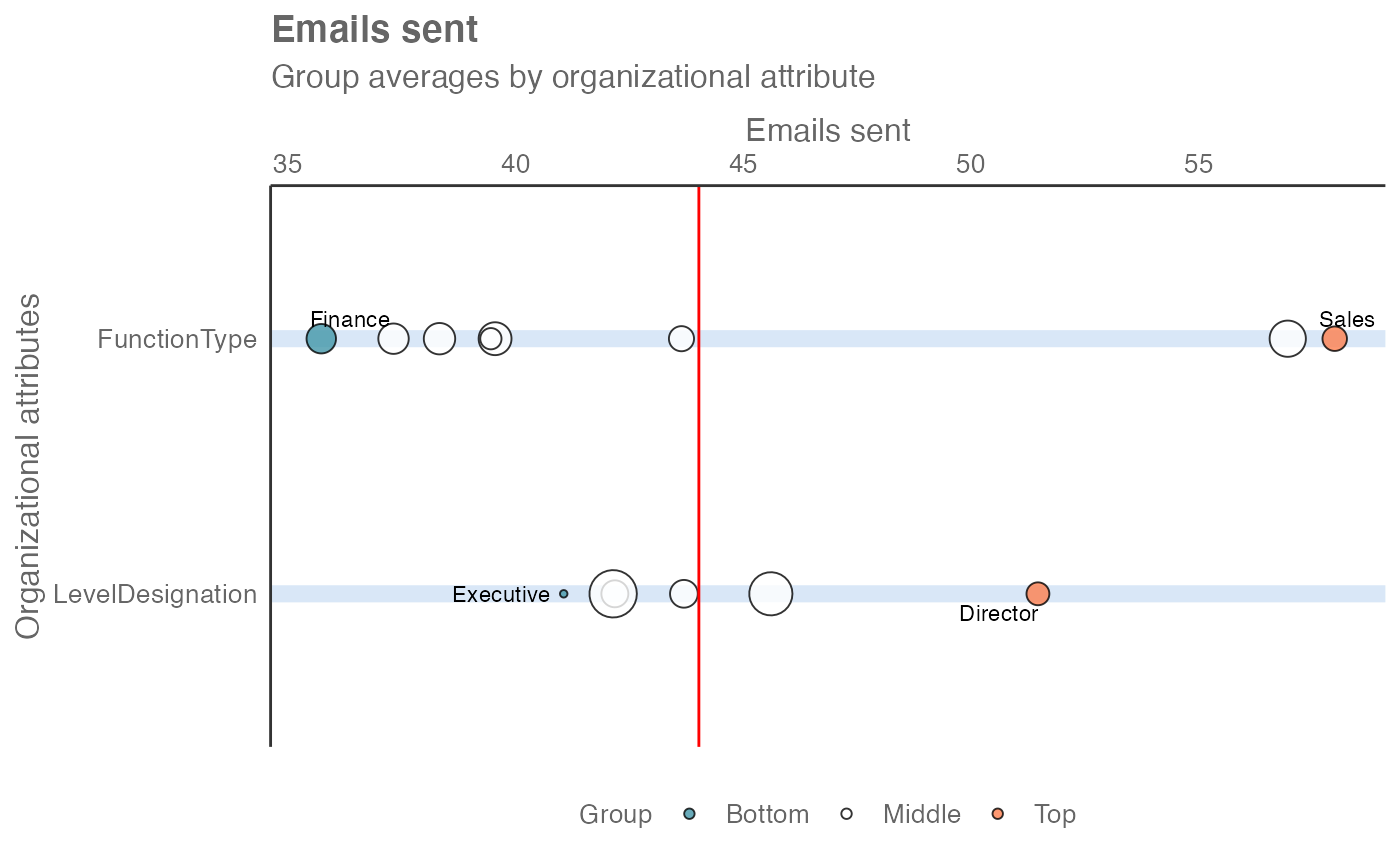
1or2, and is only used whenreturn = "plot".1: Top and bottom five groups across the data population are highlighted2: Top and bottom groups per organizational attribute are highlighted
Value
A different output is returned depending on the value passed to the return
argument:
"plot": 'ggplot' object. A bubble plot where the x-axis represents the metric, the y-axis represents the HR attributes, and the size of the bubbles represent the size of the organizations. Note that there is no plot output ifmodeis set to"combine"."table": data frame. A summary table for the metric.
See also
Other Visualization:
afterhours_dist(),
afterhours_fizz(),
afterhours_line(),
afterhours_rank(),
afterhours_summary(),
afterhours_trend(),
collaboration_area(),
collaboration_dist(),
collaboration_fizz(),
collaboration_line(),
collaboration_rank(),
collaboration_sum(),
collaboration_trend(),
create_bar(),
create_bar_asis(),
create_boxplot(),
create_bubble(),
create_dist(),
create_fizz(),
create_inc(),
create_line(),
create_line_asis(),
create_period_scatter(),
create_sankey(),
create_scatter(),
create_stacked(),
create_tracking(),
create_trend(),
email_dist(),
email_fizz(),
email_line(),
email_rank(),
email_summary(),
email_trend(),
external_dist(),
external_fizz(),
external_line(),
external_network_plot(),
external_rank(),
external_sum(),
hr_trend(),
hrvar_count(),
hrvar_trend(),
internal_network_plot(),
keymetrics_scan(),
meeting_dist(),
meeting_fizz(),
meeting_line(),
meeting_quality(),
meeting_rank(),
meeting_summary(),
meeting_trend(),
meetingtype_dist(),
meetingtype_dist_ca(),
meetingtype_dist_mt(),
meetingtype_summary(),
mgrcoatt_dist(),
mgrrel_matrix(),
one2one_dist(),
one2one_fizz(),
one2one_freq(),
one2one_line(),
one2one_rank(),
one2one_sum(),
one2one_trend(),
period_change(),
workloads_dist(),
workloads_fizz(),
workloads_line(),
workloads_rank(),
workloads_summary(),
workloads_trend(),
workpatterns_area(),
workpatterns_rank()
Other Flexible:
create_bar(),
create_bar_asis(),
create_boxplot(),
create_bubble(),
create_density(),
create_dist(),
create_fizz(),
create_hist(),
create_inc(),
create_line(),
create_line_asis(),
create_period_scatter(),
create_sankey(),
create_scatter(),
create_stacked(),
create_tracking(),
create_trend(),
period_change()
Examples
sq_data_small <- dplyr::slice_sample(sq_data, prop = 0.1)
# Plot mode 1 - show top and bottom five groups
create_rank(
data = sq_data_small,
hrvar = c("FunctionType", "LevelDesignation"),
metric = "Emails_sent",
return = "plot",
plot_mode = 1
)
 # Plot mode 2 - show top and bottom groups per HR variable
create_rank(
data = sq_data_small,
hrvar = c("FunctionType", "LevelDesignation"),
metric = "Emails_sent",
return = "plot",
plot_mode = 2
)
# Plot mode 2 - show top and bottom groups per HR variable
create_rank(
data = sq_data_small,
hrvar = c("FunctionType", "LevelDesignation"),
metric = "Emails_sent",
return = "plot",
plot_mode = 2
)
 # Return a table
create_rank(
data = sq_data_small,
metric = "Emails_sent",
return = "table"
)
#> # A tibble: 18 × 4
#> hrvar group Emails_sent n
#> <chr> <chr> <dbl> <int>
#> 1 FunctionType Sales 66.8 34
#> 2 LevelDesignation Director 62.1 24
#> 3 FunctionType Marketing 59.3 70
#> 4 LevelDesignation Manager 52.2 100
#> 5 Organization Finance 49.6 170
#> 6 Organization Financial Planning 48.3 37
#> 7 LevelDesignation Senior IC 46.2 37
#> 8 Organization Human Resources 46.1 31
#> 9 Organization Customer Service 45.9 32
#> 10 FunctionType Operations 45.0 56
#> 11 LevelDesignation Support 42.1 146
#> 12 FunctionType G_and_A 41.2 59
#> 13 FunctionType R_and_D 41.0 38
#> 14 LevelDesignation Junior IC 41.0 27
#> 15 Organization IT 40.2 67
#> 16 FunctionType Engineering 39.9 25
#> 17 FunctionType Finance 34.8 45
#> 18 FunctionType IT 31.2 10
# \donttest{
# Return a table - combination mode
create_rank(
data = sq_data_small,
metric = "Emails_sent",
mode = "combine",
return = "table"
)
#> # A tibble: 124 × 4
#> hrvar group Emails_sent n
#> <chr> <chr> <dbl> <int>
#> 1 Combined [FunctionType] Marketing [LevelDesignation] Direc… 80.1 5
#> 2 Combined [FunctionType] Sales [LevelDesignation] Manager 68.7 12
#> 3 Combined [FunctionType] Sales [LevelDesignation] Support 66.7 11
#> 4 Combined [FunctionType] Marketing [LevelDesignation] Manag… 63.2 27
#> 5 Combined [FunctionType] Marketing [LevelDesignation] Senio… 54.3 8
#> 6 Combined [FunctionType] Sales [LevelDesignation] Senior IC 54.1 5
#> 7 Combined [FunctionType] Marketing [LevelDesignation] Suppo… 53.4 26
#> 8 Combined [FunctionType] R_and_D [LevelDesignation] Director 51.6 5
#> 9 Combined [FunctionType] Operations [LevelDesignation] Mana… 50.2 13
#> 10 Combined [FunctionType] R_and_D [LevelDesignation] Manager 48.1 7
#> # ℹ 114 more rows
# }
# Return a table
create_rank(
data = sq_data_small,
metric = "Emails_sent",
return = "table"
)
#> # A tibble: 18 × 4
#> hrvar group Emails_sent n
#> <chr> <chr> <dbl> <int>
#> 1 FunctionType Sales 66.8 34
#> 2 LevelDesignation Director 62.1 24
#> 3 FunctionType Marketing 59.3 70
#> 4 LevelDesignation Manager 52.2 100
#> 5 Organization Finance 49.6 170
#> 6 Organization Financial Planning 48.3 37
#> 7 LevelDesignation Senior IC 46.2 37
#> 8 Organization Human Resources 46.1 31
#> 9 Organization Customer Service 45.9 32
#> 10 FunctionType Operations 45.0 56
#> 11 LevelDesignation Support 42.1 146
#> 12 FunctionType G_and_A 41.2 59
#> 13 FunctionType R_and_D 41.0 38
#> 14 LevelDesignation Junior IC 41.0 27
#> 15 Organization IT 40.2 67
#> 16 FunctionType Engineering 39.9 25
#> 17 FunctionType Finance 34.8 45
#> 18 FunctionType IT 31.2 10
# \donttest{
# Return a table - combination mode
create_rank(
data = sq_data_small,
metric = "Emails_sent",
mode = "combine",
return = "table"
)
#> # A tibble: 124 × 4
#> hrvar group Emails_sent n
#> <chr> <chr> <dbl> <int>
#> 1 Combined [FunctionType] Marketing [LevelDesignation] Direc… 80.1 5
#> 2 Combined [FunctionType] Sales [LevelDesignation] Manager 68.7 12
#> 3 Combined [FunctionType] Sales [LevelDesignation] Support 66.7 11
#> 4 Combined [FunctionType] Marketing [LevelDesignation] Manag… 63.2 27
#> 5 Combined [FunctionType] Marketing [LevelDesignation] Senio… 54.3 8
#> 6 Combined [FunctionType] Sales [LevelDesignation] Senior IC 54.1 5
#> 7 Combined [FunctionType] Marketing [LevelDesignation] Suppo… 53.4 26
#> 8 Combined [FunctionType] R_and_D [LevelDesignation] Director 51.6 5
#> 9 Combined [FunctionType] Operations [LevelDesignation] Mana… 50.2 13
#> 10 Combined [FunctionType] R_and_D [LevelDesignation] Manager 48.1 7
#> # ℹ 114 more rows
# }